For the final post in our series on upcoming developments for version 10.2, we look at line feeding. Line feeding allows line to be dynamically fed into, or out of, the active model.
OrcaFlex 10.2 is very nearly ready to be released and we expect this to happen in the next fortnight. In the meantime, we hope that this article whets your appetite!
Line feeding is the flagship feature of version 10.2. The new functionality is superficially similar to the OrcaFlex winch object. The winch object is a massless spring/damper whose length can vary dynamically. Line feeding also allows length to be varied dynamically, but, because it is implemented using the line object, can model mass, drag, bending stiffness etc.
This ability to dynamically vary the length of lines has been requested by users for at least as long as I have been working with OrcaFlex, over 20 years! If the functionality was easy to develop, we would have done so a long time ago. However, it is one of the most tricky developments that we have ever worked on, and has only been made possible by recent improvements to the code architecture.
What makes line feeding difficult to implement is the need to introduce new elements into the dynamic simulation, during the simulation. Apart from certain very specific scenarios it is not possible to introduce new elements, i.e. re-discretise the model, without simultaneously introducing transient loading. The main challenge for us during the development of line feeding has been to minimise these transient loads. The good news is that for the selection of cases that we have experimented with, the line feeding algorithms that we have implemented have proved to be robust.
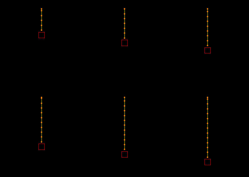
To give the above text a little context, the animation below demonstrates nodes being feed into a line to effect a lowering operation:
The data to specify line feeding is quite simple. For the example above it looks like this:
This particular line is specified to be 180m long, with 5m segment length. However, the initial arc length of End A (the top) is defined to be at 160m. Only 20m of line are active at the start of the simulation, the section between 160m and 180m. The nodes between 0m and 160m do exist internally, they are just inactive.
The payout rate of 0.2m/s defines the rate at which line is fed into the model. After 5s of simulation, 1m of line has been fed in and the arc length of End A is now 159m. The first segment is grown during the simulation to achieve this. After 25s of simulation, 5m of line have been fed into the model, and an inactive node is activated and introduced into the model. (Note that the animation has been speeded up for visualisation purposes, so new nodes appear much more frequently in the animation than every 25s.)
The above description is much simplified, and in fact the algorithms implemented in OrcaFlex are somewhat more complex in order to minimise transient loads associated with re-discretisation of the model. However, the description is intended primarily to convey the concepts behind line feeding in OrcaFlex.
Line feeding has many potential applications, including lowering / lifting analyses, laying operations, pull-in operations, and so on. It is important to stress that line feeding often introduces extra complexity to an analysis. Accordingly, it should only be used where it brings benefits of simpler modelling approaches. For instance, many aspects of lay operations are perfectly adequately modelled without dynamic line feeding. On the other hand, pipeline or cable routing analysis may well benefit from line feeding. As always, it is important to choose the right tool for the job at hand.
This has been a very superficial look at line feeding, but hopefully the potential is obvious to seasoned OrcaFlex users. We look forward to receiving your feedback, and seeing some of the models that are built using line feeding. I know that this feature has been a long time coming, I hope you enjoy it!

