Continuing our series of posts on upcoming developments for version 10.2, we now move to an important enhancement to modal analysis. This development has aspects in common with another new feature, line statics policy, which we have discussed in an earlier post.

OrcaFlex modal analysis calculates modes for individual lines or for the entire system. The individual line option is commonly used to generate mode shapes for use in an external VIV analysis program like SHEAR7 or VIVA. Modal analysis for an individual line is based on the assumption that the line end nodes are fixed, and the remaining nodes in the line have freedom. For many riser or umbilical configurations it is perfectly reasonable to use these modes in a VIV analysis. However, there are some systems for which this approach is not appropriate, and the new coupled object modal analysis feature is intended to addresses this limitation.

A good illustration of the type of system where coupled object modal analysis is important is the hybrid riser tower. For instance, this screenshot is taken from the OrcaFlex example A03 Jumper to High Tower:

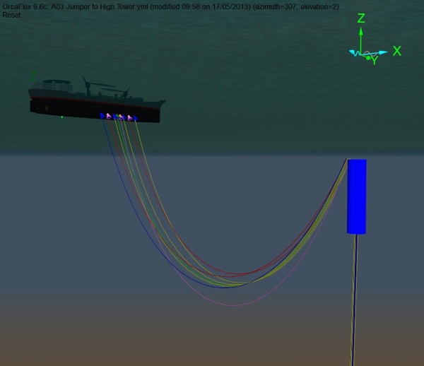
The tensioned vertical lines and the catenary lines are modelled in OrcaFlex as distinct lines and the buoyancy can is modelled with a buoy object. If we perform a modal analysis for one of the catenary lines, for instance the line named Gas, the first mode is an out-of-plane swinging mode with period 29s. The mode shape looks like this:

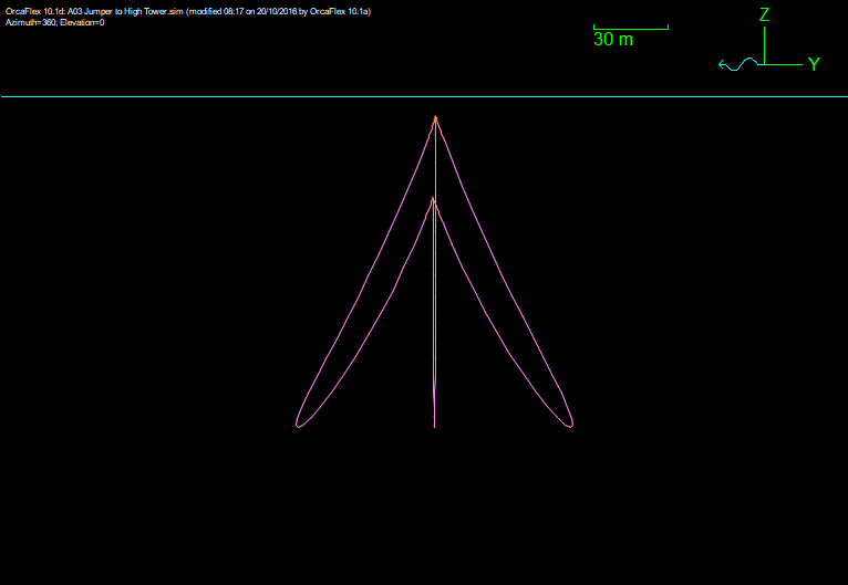
This view looks along the plane of the catenary. The mean position of the line is shown in the centre, and the lines to the left and right represent the oscillations about this mean position. Note that both ends of the line remain fixed.

By contrast if we analyse the whole system then the first mode has a period of 98s and looks like this:

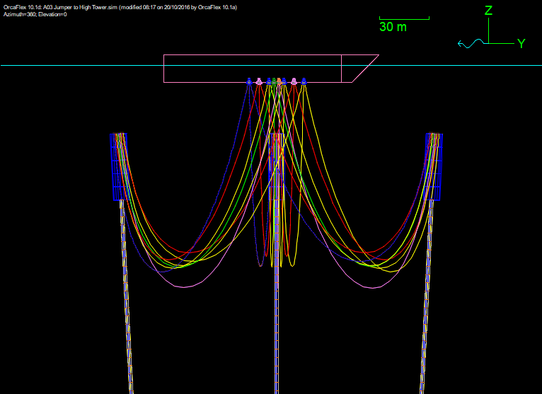
This is fairly incomprehensible at first sight, because every line in the model partakes in this mode as the lines are all coupled together by the buoyancy can. For simplicity, let’s look at the same image, but with all the catenary lines other than Gas hidden:

Again we see that the catenary line mode shape is a swinging mode, but it differs significantly in that the buoyancy can is oscillating, and hence the connected line end is oscillating. Not to mention that the mode period of 98s is more than three times greater than the individual line mode’s period of 29s!

It is therefore clear to see that when generating mode shapes for VIV analysis of such a system, we should use the fully coupled modes. In previous versions of OrcaFlex this was not possible because VIV mode shape files could only be created from individual line analyses.

So, how have we tackled this in version 10.2? Our first thought was simply to enable VIV mode shape files to be generated from a whole system modal analysis. When we considered the implications of this we came across a couple of drawbacks:

1. OrcaFlex models often contain multiple disjoint subsystems. Extending the riser tower example, consider a model with multiple riser towers. Each riser tower and connected lines form disjoint, independent subsystems. If the entire system is analysed then the output is a set of modes for the first subsystem, a set of modes for the second subsystem, and so on. It would be tricky for the program to identify automatically which modes related to the line of interest.
2. In addition to the mode identification problem outlined above, analysing the entire system could be significantly more computationally expensive than analysing a subsystem. Modal analysis for very large systems is an expensive process, and cutting the analysis down to a subsystem brings performance benefits.
3. Finally, all of our existing user interface and automation facilities for VIV modes files were line oriented rather than system oriented. It would be quite an upheaval to change that.

So, we took a different route, retaining the line oriented user interface. Using the same approach as for line statics policy, we can identify the objects that are coupled with the selected line, and perform modal analysis on that coupled subsystem. There is one very simple change to the user interface as shown below:

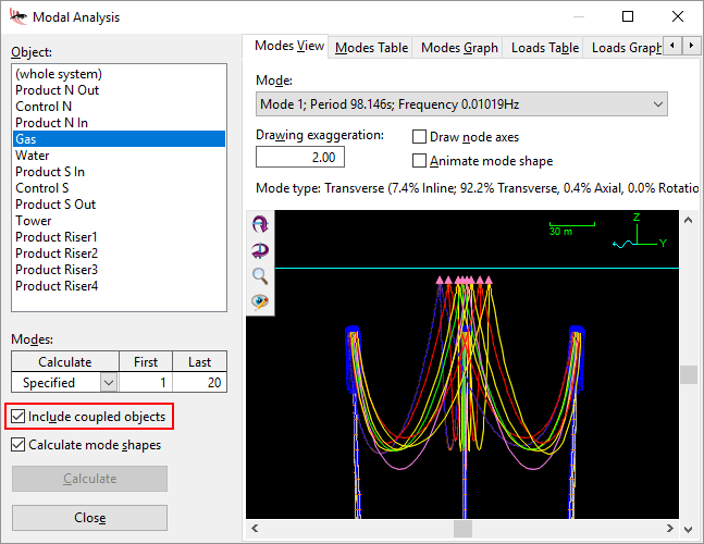
The highlighted check box enables the new functionality. When Include coupled objects is checked, the coupled subsystem containing the selected line is analysed. When unchecked, the individual line is analysed in isolation, as in previous versions of OrcaFlex.

Other areas of the program that relate to VIV modes files have also been updated. The direct SHEAR7 and VIVA interfaces now allow the choice of coupled or uncoupled modal analysis. Likewise all automation interfaces that create VIV modes files.

This has been quite a long winded article to describe a single check box! In spite of the new functionality being exposed by such a small change to the user interface, the implications of the change are significant. A large class of systems can now be analysed much more effectively than in previous versions.