Continuing our series of posts on upcoming developments for version 10.2, we look at some enhancements to static analysis.
Version 10.0 relaxed the rules for connecting objects together, one aspect of which was allowing lines to be connected to other lines. This new flexibility had a number of consequences for static analysis of lines. In version 10.0, these consequences were dealt with in a very simple manner and in many situations that approach worked perfectly adequately. However, some models that took advantage of more general connectivity proved difficult to handle in static analysis. In version 10.2 we have introduced some new functionality to address these issues.
This is quite a long and detailed post. If you don’t want to read it all, skip to the summary.
OrcaFlex statics overview
Let’s start by considering how statics analysis is implemented in OrcaFlex. The ultimate goal is to find positions and orientations for each element in the model, such that all forces and moments are in equilibrium. If the system was linear, then this could be solved directly with a single matrix solve. In practise, OrcaFlex models are invariably nonlinear and so require an iterative approach using the multi-dimensional form of Newton’s method.
Newton’s method is iterative, and requires an initial guess of the solution. It is often important for this initial guess to be close to the final solution. If the initial guess is too far away from the solution, the iteration may fail to converge to a solution, or may converge to an undesirable solution. It may sound paradoxical, but the iteration is often the easy part of the static analysis. The difficult part is choosing a good initial guess!
OrcaFlex approaches this problem in the following way:
- Fix the degrees of freedom (DOFs) of all buoys, vessels and constraints, e.g. all DOFs other than lines.
- Perform separate static analyses for each individual line.
- Release all DOFs and carry out iterative static analysis for the entire system, using Newton’s method, as described above. The outcome of the previous two steps forms the initial guess for the iteration.
Line statics
The static analysis of individual lines, which we refer to as line statics, also iterates using Newton’s method. Just as the whole system static analysis requires an initial guess, so does line statics. This initial guess is determined by the statics data on the line data form:
The step 1 method specifies how the initial guess is made. Rather than attempt to discuss every combination of this options, let us restrict discussion to the default value of Catenary. The step 1 catenary method is a discrete algorithm that, despite its name, is not based on analytic catenary equations. The method neglects bending and torsional stiffness, but does account for drag, buoyancy and seabed interaction. The method is both quick and robust and in the vast majority of cases produces a good initial guess for iterative step 2 line statics.
The step 2 method can be either None or Full Statics. The former option is used to suppress the iterative Newton’s method step of the line static analysis. This is a seldom used option and so we will ignore that option for the purpose of this discussion.
Version 10.0, lines connected to lines, all change!
The methods outlined above have proved effective over many years. However, this approach does treat lines independently from each other, at least during line statics. With version 10.0 allowing lines to be connected to other lines, it is no longer possible to treat lines independently during line statics. What to do?
For version 10.0 we tackled this in the most simple and expedient manner. We simply skipped line statics altogether for any line which had other lines connected as slaves. This allowed us to maintain the pretence that lines can be treated independently, because we only performed line statics for lines that had no dependent lines.
For many models, this approach is effective. However, by skipping line statics for master lines, we risk using a poor initial guess for whole system iterative statics. Since releasing 10.0 we have received a steady trickle of client support queries which can be characterised as statics convergence problems caused by skipping line statics for master lines. So, for version 10.2, we revisited this issue and have made improvements.
Version 10.2, line statics policy options
Rather than change the static analysis algorithms unilaterally, we have chosen to provide options to allow the user more control. Whilst having more control may sound like a good thing, it comes with a cost. The user simply wants OrcaFlex to find a static equilibrium, and in an ideal world would prefer not to care how that is achieved. Where possible we try to avoid asking the user to make such choices. If we are confident that a particular choice is always better then we hard code that into OrcaFlex and avoid asking the user to decide. However, in this instance, OrcaFlex cannot take the decision for the user because the various different options are better or worse for different models.
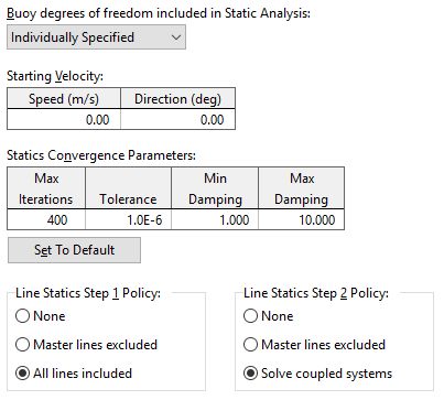
Having talked about why we are providing choice, let us now look at what that choice is. Here is the statics page of the general data form in version 10.2:
The new data are the two radio groups at the bottom, that specify step 1 and step 2 policies. The settings that are shown above, all lines included in step 1 and coupled systems solved for step 2, are the default values for new models. When old data files (created by version 10.1 and earlier) are loaded, both of these options are set to exclude master lines, because that matches the behaviour of the older versions of OrcaFlex used to create these files.
Step 1 policy
Prior to version 10.2, each line statics was performed in its entirety for each line in turn, for instance:
- Line 1, step 1
- Line 1, step 2
- Line 2, step 1
- Line 2, step 2
- etc.
Starting with version 10.2 step 1 is performed for all lines, then step 2 for all lines:
- Line 1, step 1
- Line 2, step 1
- etc.
- Line 1, step 2
- Line 2, step 2
- etc.
This change in is necessary to account for connections between lines. The options for step 1 policy are:
- None
- Master lines excluded
- All lines included
We don’t expect that None will be widely used. It has the effect of skipping step 1 statics entirely and moving to step 2 with the lines in their reset configuration. Normally this is not desirable, but there are situations where it may be more productive to move straight from the reset configuration to whole system statics. This option, and the corresponding one for step 2 make that possible.
The master lines excluded option results in the same behaviour as 10.1 and earlier.
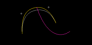
That leaves the all lines included option which is the most notable new functionality. Consider the two lines shown in this view:
Here the pink line is a slave of the yellow line. This implies an ordering for the step 1 line statics calculation. The master line (yellow) must be solved first, because the result of that solution determines the end position for the slave line (pink). More generally OrcaFlex maintains a partial order of the lines that reflects the master/slave dependencies. For any line in the model, its master lines are always to the left in this partial order, and its slave lines are always to the right. OrcaFlex uses this partial order to ensure that step 1 line statics for master lines is always performed before their slave lines.
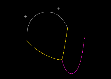
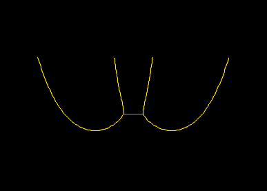
As a more compelling example, let us consider the same two lines, but with the master line using a spline starting shape. In reset state:
Then, after step 1 statics:
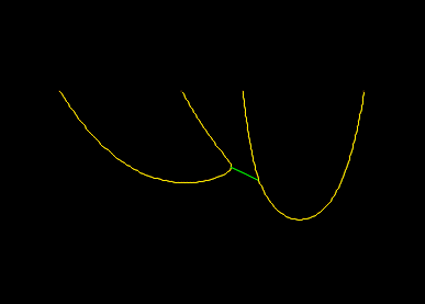
Because the yellow line is the master, its step 1 solution is performed first. This in turn determines the end position for the pink line. The true equilibrium for these coupled lines looks quite different however:
Why is this so different from the configuration after step 1? The reason is that the step 1 calculations have no coupling of loads. Without the coupling of loads, there is no mechanism for the pink line to pull the yellow line down. A consequence of this is that you may well encounter cases where the all lines included option produces a poor initial guess for step 2 line statics, and one of the other options may be more effective.
Step 2 (full statics) policy
The options for step 2 policy are:
- None
- Master lines excluded
- Solve coupled systems
You can use None to suppress step 2. This is seldom the best choice, but there are times when it can be useful. Again, the master lines excluded option reproduces the behaviour of 10.1 and earlier.
The solve coupled systems is the option of most interest to us here. When we were initially planning this development, we considered a similar approach to the all lines included step 1 option. Although, instead of working from masters through to slaves, it makes more sense to work in the opposite direction, starting with slaves, and then moving on to masters.
However, in order for the coupling between the lines to be accounted for whenever OrcaFlex is solving step 2 statics for a master line, it must include the DOFs of all slaves, including slave lines. This could lead to some undesirable consequences. For instance, consider a model with three lines: A which is a master of B which in turn is a master of C. The policy described above would lead to the following analysis sequence for line statics:
- Step 1: A
- Step 1: B
- Step 1: C
- Step 2: C
- Step 2: B, C
- Step 2: A, B, C
We realised however, that this approach has a few drawbacks. The main disadvantage is that for very long connectivity chains, this approach would be wasteful in computation. So instead, OrcaFlex inspects the connectivity between the lines and perform step 2 static analysis on each disjoint connected sub-system. So, for the example above the analysis sequence becomes:
- Step 1: A
- Step 1: B
- Step 1: C
- Step 2: A, B, C
The documentation for the solve coupled systems option expresses it like this:
OrcaFlex will attempt to identify coupled groups of lines and perform step 2 statics on each of these groups as a whole. Groups are identified by considering both the connectivity between objects and any potential stiffness terms between the degrees of freedom of the model.
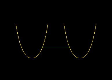
Note that as well as the connectivity, coupled groups of lines are identified by potential stiffness terms. Consider two lines, not connected directly to each other, but coupled together via a spring in the form of an OrcaFlex link object:
This spring constitutes a potential stiffness term and so when the solve coupled systems option is selected, the two lines will be solved in step 2 line statics as a single coupled group. That leads to this solution:
In older versions of OrcaFlex, or if the master lines excluded option is selected, then step 2 line statics does not consider the coupled system. Only one of the lines is influenced by the spring, and the step 2 line statics solution is:
It is worth stressing that we are still considering line statics only. Remember that this is used to form an initial guess for the whole system static analysis. So even with the uncoupled step 2 solution seen above, the whole system static analysis will consider the coupled system, and reach a coupled solution. These new line statics policy options are primarily intended to produce better initial guess for the whole system static analysis. The goal is to make statics convergence more robust and reliable, not to change the ultimate equilibrium position.
Step 2 (full statics) convergence parameters
As is often the case, many of the issues we face when implementing new functionality concern fitting in with historical precedent. Previously, step 2 line statics involved separate solves for each individual line, and each individual line had its own convergence data for step 2. With the advent of step 2 statics for groups of lines, we needed to determine the convergence parameters for a coupled solve. Rather than introduce yet more data, we decided to use the full statics convergence parameters for a specific line in the group. This is described by the documentation thus:
The Full Statics calculation for the group takes its convergence parameters from the first line appearing in the model browser (when viewing by object type) that is not a slave of any of the other lines in the group. The line whose convergence parameters are used will be the first line named in the description of the group as it appears in the statics progress window.
The statics progress window for the model considered above (two lines connected by a spring) looks like this:
Calculating static position...
Line2: Catenary statics successful
Line1: Catenary statics successful
Calculating Full Statics for [Line1, Line2]
[Line1, Line2]: Full statics successful
Converged with error = 279E-12 at Line2 node 28 Z (tolerance = 1.00E12)

Statics calculation successful
Here the two lines are group together as [Line1, Line2] and the coupled step 2 solve uses the convergence parameters of Line1.
Summary
OrcaFlex 10.2 introduces two new data items which give fine grained control of the line statics algorithms. These new options are especially valuable in systems with coupling between lines, either through direct connectivity or indirect coupling through springs. The new functionality is intended to make statics convergence more robust.
When loading data files prepared with older versions of OrcaFlex, the line statics policy data are set to reproduce the behaviour of older versions. If you wish to take advantage of the new algorithms, then you must modify that data accordingly.
Whilst we have covered these topics in a large amount of detail, you will typically be able to leave the new data at the default values, and the static analysis will be fast and reliable. Only if you encounter especially troublesome convergence problems should you need to look more deeply into the algorithms controlled by the line statics policy data.
Finally, I realise that this has been a longer than normal article. Congratulations if you made it all the way through – I promise that the next one will be shorter and more easily digestible!

