Another year passes, another OrcaFlex release arrives. After a couple of years where the release date drifted later into the year, this time around we managed to finish version 9.7a in September. All clients with up-to-date MUS contracts will have received the software by now.

Version 9.7a contained a number of minor bugs. To address these we have just released 9.7b which should be used in preference to 9.7a. The update to 9.7b can be downloaded from our website.

The enhancements introduced in 9.7 include the following:

• Sea state RAOs to model wave field disturbance effects
• Multi-body analysis, hydrodynamic interaction of multiple bodies in close proximity
• Improved vessel type data import
• New code checks: DNV OSF101/201, API RP 1111, PD 8010
• Post-calculation actions

These are just the most significant developments. As always there are a great many more enhancements which are documented in the What’s New topic for 9.7.

What follows are brief introductions to the new features that we consider to be most significant.

Sea state RAOs

Since the very first version of OrcaFlex, the program has modelled gravity waves, and their influence on the response of structural objects in the model. However, until now, waves simply passed through vessel objects as though the vessel was not present. Of course, that’s not what happens in the real world – the presence of the vessel will modify the wave field.

The effect is widely used offshore to aid lowering and lifting operations. The operation is performed in the lee of the vessel so that the vessel can act as a shield and so reduce the severity of the hydrodynamic loading on the object being lowered or lifted.

OrcaFlex 9.7 is capable of analysing this shielding effect. It would be wonderful if the program could do this for you automatically, but things are seldom that simple. The new functionality does require data. Specifically you must supply what we are terming sea state RAOs. These data are associated with a vessel type and specify the disturbance to the velocity potential. The data are quite complex, depending on heading and frequency of the incoming wave component, and on position relative to the vessel. The data are specified in a table on the vessel type form:

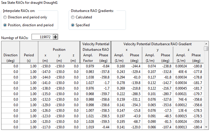
There’s a lot of data in this example, circa 120 thousand rows! This data comes from a WAMIT diffraction analysis and at the moment WAMIT is the only diffraction package from which OrcaFlex can import sea state RAO data. I won’t try to explain the data in any more detail here – I refer you to the documentation for that.

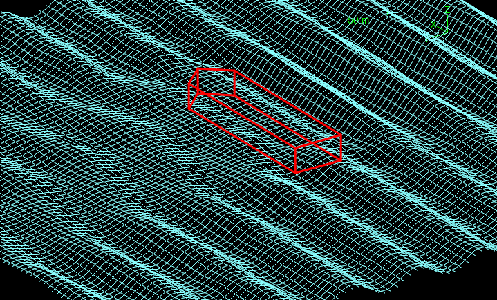
As a final parting shot, this is what the sea surface looks like when the disturbance data above are applied to a single regular wave:

Multi-body hydrodynamic interaction

This major enhancement of the calculated vessel motions capability enables the modelling of hydrodynamic interaction between two or more bodies in close proximity to each other.

To take advantage of this new feature requires a multi-body diffraction analysis. Many diffraction analysis tools are capable of performing such analyses and OrcaFlex can directly import the output from WAMIT or AQWA analyses.

Much of the data required by OrcaFlex is unchanged. For example, the format of the wave load RAOs, second order QTFs etc. is unchanged from single-body analyses. Obviously the values of these data will differ between single-body and multi-body diffraction analyses.

The main area of change are the frequency-dependent added mass and damping matrices. For single-body analyses these matrices are 6×6 in size. For multi-body analyses these matrices become 6N×6N where N is the number of bodies. The off-diagonal 6×6 blocks represent the hydrodynamic coupling in added mass and damping.

In order to support this new feature, a new object type has been introduced: the Multi-body Group. This object specifies the N vessel type/draught pairs that represent the N bodies in the multi-body diffraction analysis.

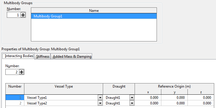
The other pages on the data form allow for specification of the hydrostatic stiffness and the frequency-dependent added mass and damping matrices. The new capability should be pretty straightforward to use as it is a simple extension of the existing capabilities.

Vessel type data import

One key facility that makes the aforementioned multi-body analysis simple to use is the ability to import data from an external diffraction package. When we came to implement multi-body analysis we realised that the existing hydrodynamic data import had a rather limited user interface. So, mainly in order to support multi-body, we re-designed the user interface. This re-design has, in our opinion, the happy side-effect that the user experience is improved even for single-body diffraction data.

The re-vamped import facility is invoked by clicking the Import button on the vessel type data form. You are first asked to select the file from which you wish to import data. After doing that the program shows the new import data dialog:

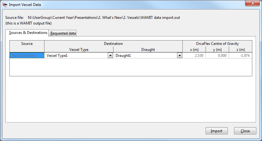
The first page, Sources & Destinations, shows you the sources (the bodies in the diffraction analysis), and the destinations (the vessel type and draught in the OrcaFlex model). If you are importing data from a multi-body diffraction analysis then multiple rows will be shown in this table.

The next step is to look at the Requested data page:

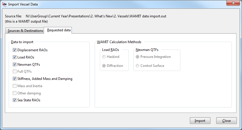
This page allows you to control what will be imported. There are various different types of data that can be imported, shown in the left hand group box. Not all diffraction analyses will include all possible types of data and those that are not available are disabled. For example, this file does not contain data for Full QTFs, Mass and Inertia and Other damping. You may decide only to import a subset of all available data. For instance, perhaps you only wish to import Displacement RAOs. In which case you would uncheck all the other options before importing.

The information on the right hand side of the page is specific to WAMIT import. Some WAMIT files contain different versions of the same data, differing only in the method used to calculate the data. For instance, Newman QTFs may be calculated by either the Pressure Integration or Control Surface method. As it happens, the file used in the example above contains only the Pressure Integration variant and so the radio group is disabled. If both options were present in the file, then you would be asked to choose one of them,

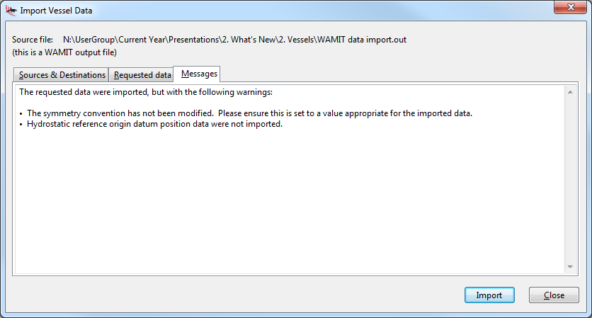
The final step is to go ahead and perform the import, which is done by the rather obvious step of clicking the Import button! The program then imports the data and shows a new page with any information messages relating to the import procedure:

We hope that the newly designed user interface will give a better experience to users.

Code Checks

Back in 2009 for version 9.3 we added an implementation of the stress checks from the API RP 2RD riser design code. Back then, we added a section of line type data named Code Checks and used the plural form (as opposed to writing Code Check) because we anticipated adding more codes in the near future.

Well, that “near future” turned out to be four years later with 9.7! We have added a number of new design code checks to the program. The list of implemented codes is:

• API RP 2RD
• API RP 1111
• DNV OS F101
• DNV OS F201
• PD 8010

Previous versions placed the API RP 2RD data on the line type data form. With 9.7 we now have so many code checks implemented, and with so much extra data, that we decided to move the data onto a separate data form.

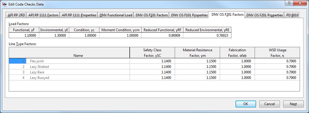
The code check data is needed to specify information that is required by the design code, but not by the OrcaFlex simulation.

The new functionality is purely an exercise in post-processing. Each design code has associated with it a series of results variables. Typically these variables are presented as unity checks. That is, a value less than one means that the code is satisfied, otherwise the code has been infringed. These results variables are standard OrcaFlex results variables and so you can extract time histories, range graphs, statistics etc. These code check results can be post-processed using all the standard OrcaFlex automation facilities.

Implementing these new code checks was not a trivial task. The design code documents are sometimes quite tricky to understand and interpret. We hope that we have managed to interpret them correctly. However, as a user you should make sure that the implementation in OrcaFlex agrees with your interpretation of the code. Not least this will be needed in order for you to supply the input data. Accordingly we have provided comprehensive documentation of our implementation.

Post-calculation actions

Post calculation actions are a new way to perform post-processing. The feature allows you to specify the post-processing in the OrcaFlex data file. There are a number of reasons why this may be attractive, including:

• It allows you to perform post-processing immediately after the simulation and without having to re-load the simulation file.
• If for whatever reason you do not like Excel, then this gives you an option to have your post-processing invoked as part of the standard OrcaFlex automation.
• Even if you do like to use Excel, there’s no way to invoke Excel post-processing from Distributed OrcaFlex.

The post-calculation actions are specified on the General data form:

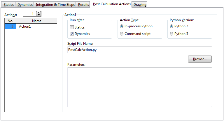
Note that you can specify multiple actions, although we expect that you would rarely specify more than one. You can specify that actions run after static, after dynamics, or after both statics and dynamics. Again, we expect that they would most commonly be executed after dynamics as shown above.

The post-calculation action itself can be defined either as a Python script, or as a command script. The latter is more general, allowing you to call any other process. However, the command script option runs the post-processing in a separate process and so will require that process to load up the simulation file. For this reason, and others, the in-process Python option is strongly recommended.

So, what does a post-calculation action script look like? The example below, taken from the documentation, is just about the simplest script possible:

import os.path

def Execute(info):
line = info.model['Line1']
tension = line.TimeHistory('Effective Tension', objectExtra=OrcFxAPI.oeEndA)
outputFileName = os.path.splitext(info.modelFileName)[0] + '.txt'
with open(outputFileName, 'w') as f:
f.write(line.name + ' End A Effective Tension\n')
for value in tension:
f.write(str(value) + '\n')

The script is passed information in the info parameter. The script can access the model and its objects through info.model. The script can also obtain the simulation file name through info.modelFileName which is used above to generate an output file name that matches the simulation file name. This allows you to use the same script for multiple different simulation files which is clearly desirable.

The rest of the code should be fairly obvious to anyone with experience programming against the OrcaFlex Python interface. The script extracts a time history of Effective Tension for the object named Line1 and then writes that to a file.

Clearly this is a very basic and simple example, but there is no limit to what your scripts could do. Any post-processing that can be achieved using the OrcaFlex Python interface can be performed in a post-calculation action.

Finally, how are these actions executed? They are designed to be performed as part of your automation workflow. Hence they do not run when you perform interactive calculations. Post-calculation actions are executed when a calculation is performed either using the OrcaFlex batch form, or from Distributed OrcaFlex.

Conclusion

So, that’s OrcaFlex 9.7. We hope you enjoy it, and find good use for all the new features. We are already busy working on 9.8 which you can expect to see in the second half of 2014.