We are very pleased to announce the release of OrcaFlex version 11.1. The software was finalised and built on 12th February. We originally planned to release 11.1 in Q4 of 2020. However, we delayed the release in order to complete the restart analysis development. We plan to make the next release in the traditional Q4 slot, later this year.
All clients with up-to-date MUS contracts will receive, in the week starting 22nd February, an e-mail with instructions on how to download the new version.
Version 11.1 introduces much new functionality, including:
- Restart analysis, variation models, and change tracking
- Turbine pre-bend
- Turbine range graphs
- Hysteretic and externally calculated axial and torsional line stiffness
- Performance improvements for wave time history analysis
- Wire frame drawings specified by panels
- Embedded Python scripts as an alternative to external files
- OrcaWave intermediate results
- OrcaWave target roll damping
- OrcaWave performance improvements
These are the most significant developments, in our opinion. As always there are more enhancements that are not listed here. All new features are fully documented in the what’s new topics:
What follows is a brief introduction to each of the new features that we consider to be of most significance.
Restart analysis, variation models, and change tracking
Restart analysis is a common feature in many finite element codes, but for various historical reasons, OrcaFlex has not implemented restart analysis until now.
In a restart analysis, the initial conditions and state are determined by the output of a prior analysis (which we refer to as the parent analysis). Model data may be modified in a restart analysis. In order to define a restart analysis we need the following:
- A parent data file (.dat or .yml) that defines the input data for the parent analysis.
- A parent simulation file (.sim) that is used to determine the initial conditions of the restart analysis.
- A restart data file (.yml) that defines the modifications to the input data for the restart analysis.
Because a restart typically changes only a small number of data items, we want the restart data file to contain only the data that is different from the data in the parent. To achieve this we have extended our existing YAML text data file format. These text data files can define the entire data for a model, but more commonly they are used to make a small number of data changes to a base model. We refer to this as a variation model. Here is a simple example:
BaseFile: base.dat
Environment:
  WaveTrains:
    Wave1:
      WaveHeight: 5
      WavePeriod: 9
The model defined by this file is the same as base.dat, but with changes made to the wave height and period.
In previous versions of OrcaFlex you had to create these variation files manually in a text editor. And when you loaded these files in OrcaFlex the data changes were applied but the program did not keep track of the changes.
Starting with 11.1, OrcaFlex now implements change tracking. When the above model is loaded, the environment data form looks like this:
![]()
As you can see, the modified data items are highlighted on the data form. Because the program can now track changes, you can build variation files directly in OrcaFlex without having to use a text editor. This makes it much easier to build variation files which is a powerful enhancement to the program in its own right.
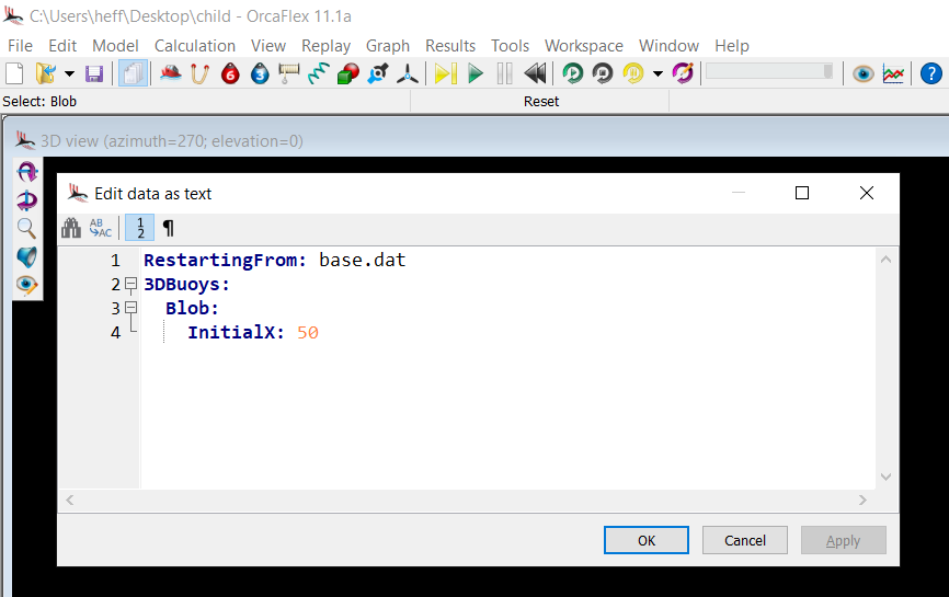
Restart files are very similar, differing only in the use of RestartingFrom instead of BaseFile. For example:
RestartingFrom: parent.yml
3DBuoys:
  Blob:
    InitialX: 50
This makes a single change to the data inherited from the parent model. When editing the data in the GUI, this change is highlighted on the object data form:
![]()
The change of the initial X position to 50 is highlighted in red. The other two positions are highlighted in blue which means that the values will be ignored, and instead the latest position from the parent analysis will be used as the initial Y and Z positions.
The model data can even be edited (in text format) from inside the program with a built-in text editor.
This feature can be used to find which data have been modified. Mass changes can quickly be made by editing the text.
We’ve seen how to create the input data for a restart analysis, and the final piece of the jigsaw is the restart analysis calculation. OrcaFlex allows all combinations of statics and dynamics restarts. You can perform a static restart from a static or dynamic parent analysis, and you can perform a dynamic restart from a static or dynamic parent analysis. Whilst almost all data can be changed in a restart analysis, not all changes will make physical sense. However, we have tried hard to make the feature as flexible as possible.
When a restart analysis starts, the parent simulation file is loaded and all state that can be mapped from the parent analysis to the restart analysis is transferred.
Restarts can be useful for a variety of modelling tasks that would otherwise be difficult or impossible to achieve. Examples include:
- Sometimes one has a suite of models that differ only in their dynamic behaviour, but whose static configuration is common to all the models in the suite. If the statics calculation is slow to converge and takes a long time to run, then a lot of time will be wasted repeating the calculation when batch processing the entire suite. With restart analyses, the static calculation can be performed once only, in a parent model, and then multiple dynamic-only child models can restart from this (each one loading the same static state parent simulation file, rather than recalculating).
- Although OrcaFlex has many features to improve statics convergence, some models can still present significant challenges for static analysis. A series of static restart analyses can often be used to resolve such problems. For instance, you might apply a vessel offset in a series of static restarts, and then introduce current in the final static restart.
- Restarts can be used to build up a friction history in a series of successive static analyses. Each analysis would perturb the previous one in a small way (e.g. by slowly changing the current in the model, or dragging the end of a line to a slightly different location), gradually building up to the final static equilibrium required, in a way that more accurately accounted for frictional forces than a single standard analysis.
- The same concept could be applied to other history dependent load models, e.g. hysteretic line stiffness (axial, bending or torsional), hysteretic constraint stiffness, nonlinear soil model, etc.
We are quite sure that this list only scratches the surface of what can be achieved with restarts and are looking forward to discovering what other uses you find for restarts.
OrcaWave
OrcaWave is our diffraction / radiation code, released last year with 11.0. Since that initial release we have continued to develop it.
Mesh file formats
Over the course of the 11.0 minor updates we have added support for a host of new mesh file formats (Hydrostar, Aqwa, Sesam, Gmsh) and these formats have also found their way into OrcaFlex panel mesh import for drawing.
Performance
When we released 11.0 we were aware that there were a number of opportunities to improve the performance for OrcaWave. We ran out of time to implement these in that initial release, but have subsequently made significant improvements. In 11.0d we introduced an iterative linear solver, as an option alongside the direct linear solver. In 11.1 we have further optimised both iterative and direct linear solvers, but especially the direct solver. Broadly speaking, the iterative solver is faster for larger meshes, and the direct solver is faster for smaller meshes. The direct solver that we now use is so fast, that the tipping point, where iterative starts to out-perform direct, is reached only for very large meshes. So, at least in our experience, we expect that the direct solver is usually preferable now.
As well as all the work on solvers, we have identified other performance bottlenecks and optimised that code. We have also reduced memory usage and added a report of expected memory usage.
Intermediate results
OrcaWave can now perform analyses that make use of a previously performed analysis. The idea is that the time-consuming step of populating and solving the first-order boundary integral matrix equations is performed once, and then subsequent analyses can avoid repeating this calculation.
This is only possible if the input data on which first-order solution depends matches between the parent and child models. This is data such as body mesh, wave periods, water depth, etc. Data that may be modified in the child model includes:
- Inertia or constraints data for one or more bodies.
- Control surface mesh files for one or more bodies.
- Free surface data in a full QTF calculation relating to the panelled, quadrature and asymptotic zones.
In the next release of OrcaWave we will introduce features to perform stochastic linearisation of quadratic Morison drag loading. This is another feature that benefits from intermediate results, allowing you to perform the stochastic linearisation without having to repeat the first-order calculation.
Roll damping target percentage (for free-floating ship shaped bodies)
Roll damping results have been added which show the level of roll damping, relative to critical, for each body. A new data item allows you to specify a target percentage, in which case OrcaWave will increase the external roll damping coefficient to meet the target.
Interior surface panels
If your body mesh does not include interior surface panels (used to remove irregular frequency effects), then you can ask OrcaWave to automatically generate interior surface panels. In 11.1 we have added a new option for that automatic generation. The previous method is known as the radial method, and the new method is triangulation.
The new triangulation method often performs better for waterlines with a large aspect ratio (e.g. a typical ship) and it can also handle highly concave waterlines, for which the radial method breaks down.
Improved waterline detection
We have made a number of improvements to the waterline detection algorithm.
Can optionally divide non-planar quads into two panels when importing meshes
There is a new option (on the calculation & output page) to divide non-planar panels on import from panel mesh files. If this is checked, any panels that are determined to be non-planar (projection length exceeding the length tolerance) are split into two triangles.
QTF crossing angle range and QTF period or frequency range
New data items have been added that allow you to reduce the number of second-order loads that OrcaWave will compute.
The QTF crossing angle range applies to the wave headings included in mean drift loads and full QTFs. The absolute value of the crossing angle is restricted to the specified range. The default range [0°, 180°] means all crossing angles are considered. Setting the range to [0°, 0°] restricts to unidirectional waves.
If full QTFs are being calculated, you can also restrict the range of QTF periods or frequencies considered. If the number of QTFs is significantly reduced, this can in turn reduce the calculation time.
Improvements to drawing options
A number of minor enhancements have been made for drawing.
- Body axes can be drawn.
- Wave heading directions can now be shown in the mesh view.
- Free surface quadrature zone points and outer circle points can now be drawn.
- The measuring tape tool, familiar to OrcaFlex users, is now available on the mesh view.
Turbines
Turbine blades can now be pre-bent to model blades which are not straight in their unstressed state. Modelling pre-bend can have a significant impact on the dynamic response of a turbine and so this is an important enhancement.
Range graph results are now available for turbine blades. This allows you to plot the variation of a result variable over the length of a blade, in exactly the same way as line range graphs.
Finally, we have provided a new turbine example which models the NREL 15MW reference wind turbine. This is notable because it uses the NREL reference open source controller (ROSCO).
Hysteretic and externally calculated axial and torsional line stiffness
Line bend stiffness can be specified in a number of different ways: linear, non-linear elastic, non-linear hysteretic and by external function. In previous versions, axial and torsional stiffness could be specified by either linear or non-linear elastic data. In 11.1, axial and torsional line stiffness can additionally be specified as non-linear hysteretic or by an external function.
Performance improvements for wave time history analysis
When waves are specified by elevation time history, OrcaFlex has to perform a Fourier transform of the time history to obtain a set of linear wave components to realise that time history. The number of wave components increases with the number of time history samples, and for long histories there can be a huge number of wave components. In turn, this can lead to very slow simulations because OrcaFlex gets bogged down evaluating wave kinematics.
When you inspect the wave components produced by the Fourier transform, the vast majority of them are high frequency components with tiny amplitude. In 11.1 there is now an option to remove the highest frequency components automatically. You specify the proportion of the spectral energy that is to be removed. For example, if you specify a truncation threshold of 1%, then OrcaFlex will remove the highest frequency components that sum to no more than 1% of the total spectral energy.
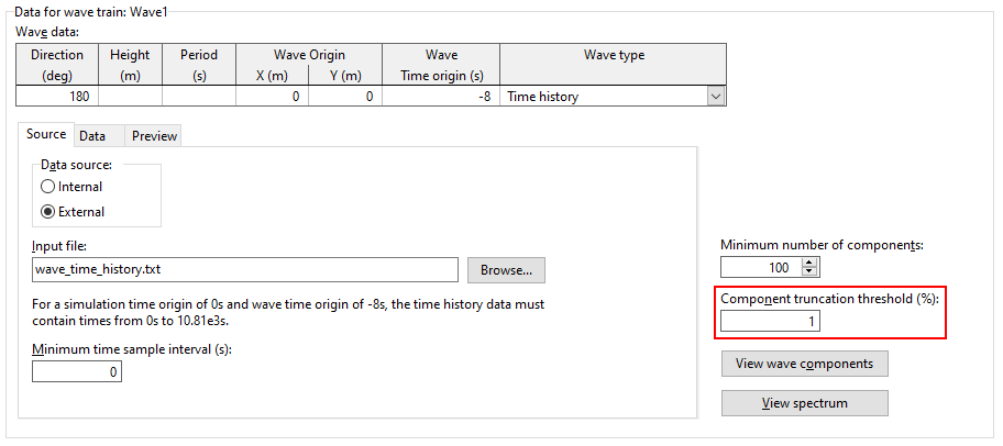
Because of the way the components are distributed, removing a small amount of the overall spectral energy typically results in a huge reduction in the number of components to be evaluated. As always, we recommend that you perform sensitivity studies to convince yourself that these optimisations don’t have a significant impact on the results of interest.
Wire frame drawings specified by panels
Wire frame drawings for buoys and vessels have historically been specified by lists of vertices and edges that define a set of line segments. When drawing in the shaded graphics mode, OrcaFlex will use these data if a separate 3D model (.x or .obj) has not been provided. In order to do this, OrcaFlex needs a set of triangular panels which it obtains from the wire frame edges by finding the smallest convex hull containing those edges.
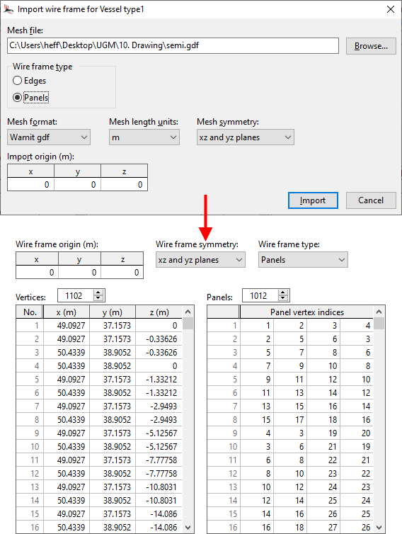
In version 11.0, primarily for use in OrcaWave, we developed code to read from a range of panel mesh files. We made use of that code in OrcaFlex, adding a feature to import such panel mesh files as wire frame drawings. In version 11.0 we converted the panel mesh into vertices and edges, since that was the format of the data in that version. However, we have subsequently realised that it would be beneficial to retain the panel information. If we do so then we do not need to calculate a convex hull when using the wire frame data in the shaded graphics mode. Not only does this save on calculation time, it means that non-convex shapes can be drawn correctly.
So in OrcaFlex 11.1 the wire frame drawing data can now be specified either by edges (as in previous versions), or by panels. The panel mesh import facility allows you to choose which specification to use (edges or panels). We would usually recommend using panels and expect that importing wire frame data as edges would only be useful when sharing data files with users who do not have access to 11.1.
In addition to specifying the data as panels, wire frame drawing data can now take advantage of the symmetries that are common in these data. This allows for more efficient storage for detailed panel mesh data.
Embedded Python scripts as an alternative to external files
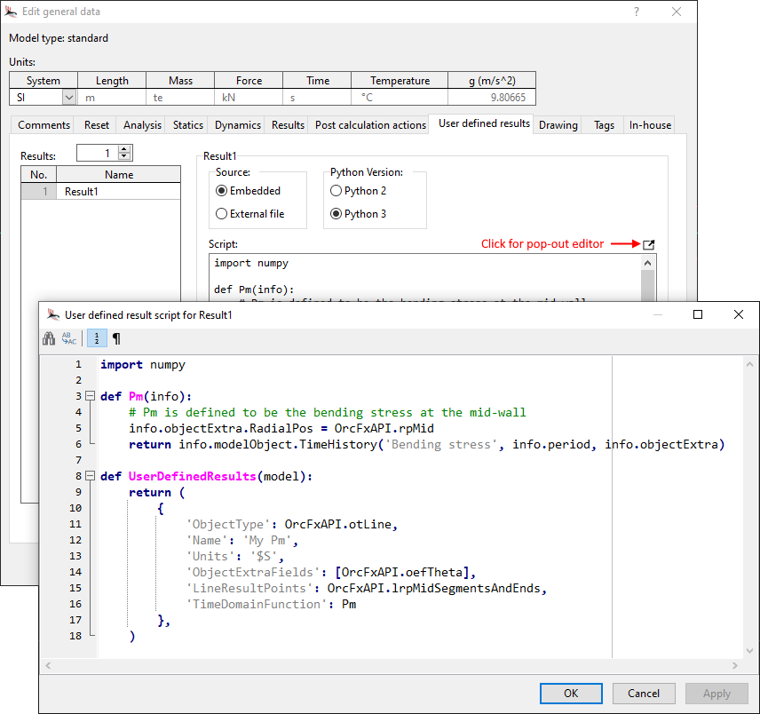
OrcaFlex has a number of features based on executing Python code specified in external Python script files. These features are external functions, post calculation actions, and user defined results. As an alternative to specifying the script in an external file, the script can now be embedded in the model data. This can make workflow easier because the input data can be entirely contained in the input data file.
As well as catering for embedded scripts, we have introduced a very basic pop-out editor which has support for syntax highlighting, code-folding etc. Note that we have no ambition to include a fully featured text editor in OrcaFlex, and so if you need more functionality than we have provided you should use an external text editor.
While having these scripts embedded can be very convenient, there are still numerous situations where external scripts may be preferable:
- If you have multiple models that all use the same script, then it is repetitive to embed it. If you have to change the script, then an external script would allow the edit to be made in that single external file.
- Sometimes it is useful to share code between different external functions. A classic example can be found in our turbine controller examples which have both pitch and generator controllers, and share code. An embedded script means two copies of the shared code, and perhaps an external script is better.
- An external script allows for revision control of the script.
This is not to say that embedded scripts are not often very useful, but it is always important to use the right tool for the job.
Conclusion
So, that’s OrcaFlex 11.1. It has been a long time in the making, and we hope that it proves to have been worth waiting for!