We are very pleased to announce the release of OrcaFlex version 11.4. The software was finalised and built on 22^nd November. All clients with up-to-date MUS contracts will receive, in the week starting 27^th November, an e-mail with instructions on how to download and install the new version.

Version 11.4 introduces much new functionality, including:

OrcaFlex

• Indirect constraints and double-sided connections
• Jacobian perturbation factor
• Turbine rotation sense, tower shadow models, downwind turbines
• Wind modelling improvements
• Tabular current velocity & acceleration
• Line/seabed contact properties can vary with arc length

OrcaWave

• Sectional bodies
• Mean drift loads via momentum conservation
• Automatic mesh generation
• Detection of field points inside a body
• External stiffness for rigidly connected bodies now calculated by OrcaWave

These are the most significant developments, in our opinion. As always there are more enhancements that are not listed here. All new features are fully documented in the what’s new topics:

• OrcaFlex
• OrcaWave

What follows is a brief introduction to each of the main new features.

Indirect constraints and double-sided connections

Constraints were introduced in version 10.1. When we originally implemented constraints, we considered two candidate methods to implement the functionality:

1. Using coordinate mappings to directly express the position and orientation of the out-frame in terms of the position and orientation of the in-frame.
2. Solve the constraint equations implicitly. This is achieved by adding additional, non-dynamical degrees of freedom to the system, Lagrange multipliers, which are closely related to the constraint forces needed to enforce the constraint equations.

There are pros and cons to both methods, but we opted to implement method 1. In version 11.4 we have introduced method 2 as an alternative. These two methods are presented in the UI as direct (method 1) and indirect (method 2).

The indirect method can be more computationally efficient, especially when many constraints are chained together, and also permits the use of double-sided connections (see below).

However, the indirect method does have some disadvantages:

• Since the constraint equations are solved for indirectly by the solver, they may only be satisfied up to the tolerance of the solve. For instance, a Cartesian constraint with its internal x degree of freedom locked out should report x = 0 at all log sample times, when asked for results upon completion of a simulation. This will be the case for directly solved constraints, but for indirect constraints there may be some small fluctuations about zero, governed by the tolerance of the analysis.
• The introduction of non-dynamical degrees of freedom can make models more prone to convergence problems, preventing them from running to completion.
• Models represented by indeterminate systems of mathematical equations are more frequently encountered when using the indirect solution method. Such a model may be perfectly valid from a physics perspective, but may produce singular Jacobian matrices because of redundant degrees of freedom perceived by the solver. Such models will fail to run, usually by raising a singular matrix error in statics. This problem can often be overcome by defining a small, but non-zero, Jacobian perturbation factor for the model, but this requires extra consideration on the part of the user when building models.
• Lagrange multipliers are not compatible with explicit time domain integration or modal analysis.
• It cannot account for rotational winding between the in-frame and the out-frame.

Double-sided connections were mentioned above, and these can now be made when using indirect constraints. These allow the in-frame and the out-frame to be independently connected to other model objects. This capability can be used to avoid issues relating to circular connection dependencies, which could otherwise hinder model building and lead to unnecessary confusion. Double-sided connections will aid in the modelling of systems composed of large numbers of interconnecting objects, such as solar arrays and sea-fastening operations.

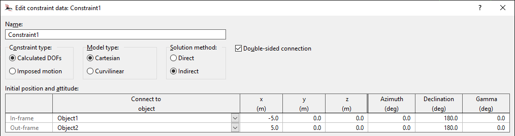
Although double-sided connections can help with modelling of complex systems, they are also extremely useful for model building, even for simpler systems. The ability to see and edit both connections in the same place makes model building much simpler. We anticipate that double-sided connections will be very widely used.

Jacobian perturbation factor

The text above mentioned the Jacobian perturbation factor, and this is a new feature introduced in 11.4. This was introduced specifically to facilitate convergence for the indeterminate systems that can arise with indirect solution method constraints. However there are other scenarios which can lead to indeterminate systems. A common example looks like this:

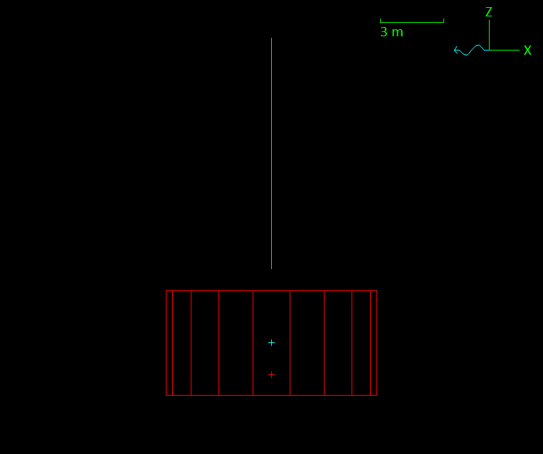
Here the buoy’s centre of mass and centre of buoyancy are inline with the spring that is supporting the buoy, and the buoy’s orientation about the Z axis is indeterminate. Calculation of statics fails with this (possibly familiar) error:

Whole system statics: Indeterminate case (singular Jacobian)

If you set a small value for the new Jacobian perturbation factor, then this error does not occur, and the statics calculation can be solved.

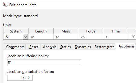
The Jacobian perturbation factor is a non-dimensional number that adds in a small additional contribution to the diagonal of the Jacobian matrix. Each additional diagonal entry is weighted by the characteristic scales of the model, so as to keep the Jacobian dimensionally consistent. Even a tiny perturbation (e.g. 10^-18) can be sufficient to resolve singular Jacobian issues and permit the analysis to proceed. In fact, the smaller the perturbation, the better: the larger the perturbation, the less closely the Jacobian matrix resembles the physical system it is meant to represent. The implications of this discrepancy depend on the type of analysis being performed:

• Statics and implicit time-domain dynamics: the solver only uses the Jacobian matrix as a guide to improve convergence in these analyses. The results will still accurate up to the user-specified tolerance, provided that convergence is ultimately achieved. If the magnitude of the Jacobian perturbation factor is too large, then the model may not converge when run.
• Explicit time-domain dynamics: the Jacobian perturbation factor has no direct effect on these analyses. However, it can alter the calculation of OrcaFlex’s recommended time-step, which can affect the model if it is used in the subsequent analysis.
• Frequency domain and modal analyses: the results from these analyses are directly dependent on the Jacobian matrix. This means that even a small perturbation will change the outcome of the analysis and extreme caution is required. It is recommended to keep the perturbation as small as possible, perhaps by conducting a sensitivity analysis.

We have set the default value for this data to be zero. This means that indeterminate systems will still result in singular Jacobian errors. We feel that it is important to be notified of this, even if you subsequently decide to use the Jacobian perturbation to avoid the singular Jacobians and accept the indeterminacy.

Turbine rotation sense, tower shadow models, downwind turbines

There are two developments in OrcaFlex 11.4 for the turbine object, both for the benefit of users modelling downwind turbines:

• The turbine’s rotation sense can now be nominated. This is the direction the rotor is expected to spin in normal operation, when viewed from upwind. It determines how the blade profile data is interpreted, how the aerodynamic load is calculated and the conventions used to interpret controller input. A conventional turbine will have a clockwise rotation sense, which was always the assumed behaviour in previous versions. However, some turbines, e.g. certain downwind turbines, rotate the other way. Previously it was very difficult to model such turbines and the blade data had to be manipulated before being entered. Now, for such rotors, anticlockwise can be chosen for the rotation sense and the blade data can be entered in a more natural format.
• The turbine now includes the Powles and Eames tower shadow models. These models are used in the tower disturbance calculation to modify the wind field to account for the velocity deficit in the wake behind the tower.

Wind modelling improvements

There have been a number of changes to the wind modelling features offered by OrcaFlex. Primarily these have been motivated by wind turbine applications. In summary the changes are:

• Wind time history files can now specify variation of speed, direction, shear and gust. This facilitates the modelling of wind fields with time varying linear shear, both horizontal and vertical, which is required to satisfy the IEC 61400-1 extreme wind shear (EWS) design load case. Previously only variation of wind speed and direction could be included.
• Full field wind files generated by the Mann turbulence generator are now supported.
• Wind ramping options (no ramping, ramp from zero, or ramp from mean) can be specified for all wind types.
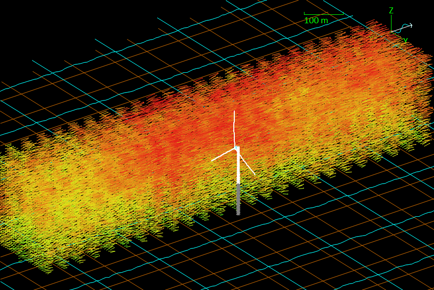
• Full field wind boxes can now be visualised in the 3D view.

Tabular current velocity & acceleration

Current velocity and acceleration can now be specified in tabular form, as a function of simulation time and position. The table can either be directly defined within OrcaFlex or provided from an external file.

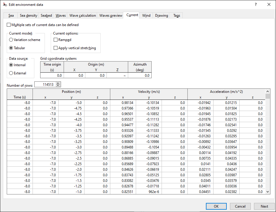
Non-zero current acceleration is a new feature; it is combined with the wave acceleration for purposes of computing Froude-Krylov and added mass loads.

Although this functionality is intended for more general current modelling, in principle it could be used to specify complete fluid kinematic fields.

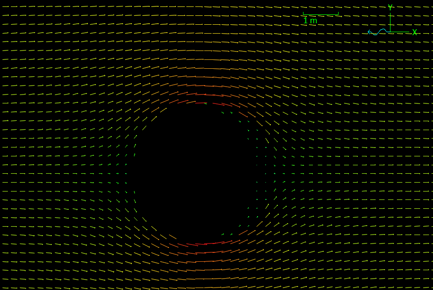
The tabular current can be visualised in the 3D view in a similar way to full field wind:

Line/seabed contact properties can vary with arc length

Seabed contact properties for lines can now be defined to vary along the length of line. This is achieved by defining seabed sections on the line data form, specified by arc length ranges. This extends the previous functionality to specify seabed resistance profiles.

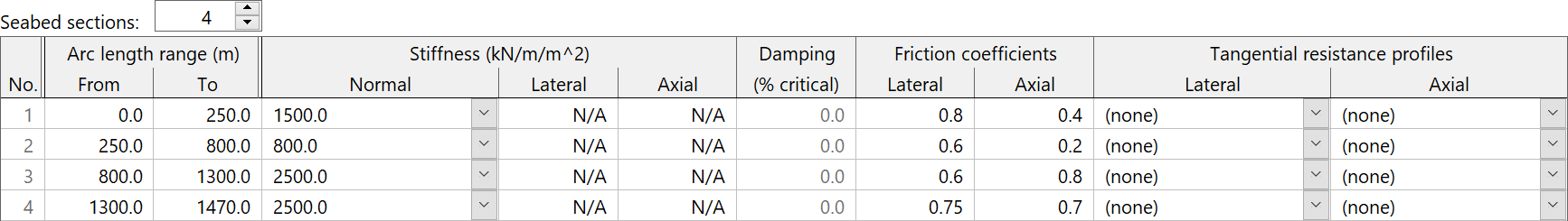
The following properties can be controlled: normal, lateral and axial stiffnesses; damping; lateral and axial friction coefficients.

In the example data above, the N/A values indicate that the global value specified on the environment data form is to be used. In addition, some of the columns accept ~ as a special value. For instance, an axial stiffness value of ~ means that the axial stiffness is the same as the lateral stiffness.

Full details of how these data are interpreted are given in the documentation.

Sectional bodies

OrcaWave can now analyse models in which a structure is divided into multiple sectional bodies – defined as bodies for which the wet body surface may be open-ended. The principal motivation is to enable multi-vessel OrcaFlex models which study dynamic connection loads within a large structure. Here is an example of a wind semisubmersible divided into seven sections, each represented in OrcaWave by an open-ended panel mesh:

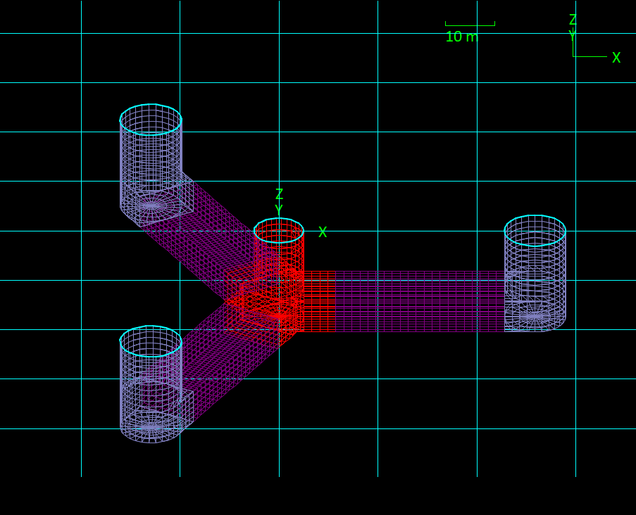
As in this example, the union of all the sectional bodies in a model must yield one (or more) closed structure in order to perform a valid diffraction analysis. But a sectional body viewed in isolation may be open ended, and this significantly changes the hydrostatic results available in comparison to a conventional body with a closed surface (which we refer to as a displacement body). The differences arise because waterlines, interior surfaces and displaced volume are all properties of the combined structure, rather than individual bodies. In particular, sectional bodies have no volume or centre of buoyancy results, while the hydrostatic stiffness matrix has more non-zero coefficients. Non-hydrostatic results, e.g. added mass and damping matrices or load RAOs, have the same form as for a displacement body.

A parallel development in OrcaFlex 11.4 allows the new hydrostatic results to be used by an OrcaFlex vessel type. Instead of the familiar data for volume, centre of buoyancy and (3 × 3) symmetric hydrostatic stiffness matrix, a sectional vessel type has a datum buoyancy load and a non-symmetric (6 × 3) hydrostatic stiffness matrix.

Mean drift loads via momentum conservation

OrcaWave can now compute mean drift loads using the momentum conservation method (also known as the far-field method).

Results are limited to horizontal (surge, sway and yaw) mean drift loads. Further, in a multibody model, it does not give loads on individual bodies. In other respects momentum conservation is closely related to control surface integration and, like that method, it often has good mesh convergence properties.

Automatic mesh generation

OrcaWave can now automatically generate meshes for control surfaces and free surface panelled zones:

• If your quadratic load calculation method includes the control surface method, OrcaWave can now automatically generate a control surface.
• If your solve type is a full QTF calculation, OrcaWave can now automatically generate a mesh of the free surface panelled zone.

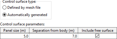
As an illustration, this is the input data for the automatically generated control surface mesh:

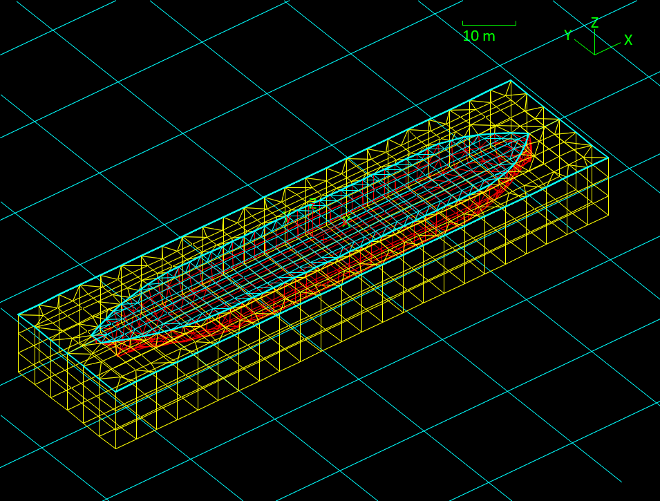
And here is a view of the corresponding automatically generated control surface mesh, drawn in yellow:

Detection of field points inside a body

OrcaWave can now detect field points that are inside a body. There is no meaningful sea state RAO result at such points because they are not in the water, so OrcaWave can optionally return a simple ? placeholder instead.

The motivation for this feature is the requirement for a complete grid of positions in the sea state disturbance RAOs of an OrcaFlex vessel type. If this requirement forces you to put field points inside a body, there is a danger that meaningless RAO results could be used during an OrcaFlex simulation. The ? placeholders from OrcaWave replace results that would otherwise have meaningless values, and a parallel development in OrcaFlex 11.4 allows them to be interpreted appropriately in OrcaFlex.

External stiffness for rigidly connected bodies now calculated by OrcaWave

OrcaWave now has a simpler workflow for building models with rigidly-connected bodies. In previous versions, external stiffness data was required to capture the effect of a mean (i.e. zeroth-order) connection load on the first-order equation of motion. That stiffness data could be obtained from mooring stiffness reports in OrcaFlex, but the workflow was unsatisfactorily complex. OrcaWave now fully accounts for the connection load, so you do not need to provide any external stiffness data as a result of specifying a connection.

Results for displacement RAOs (and quantities dependent on them) will be affected for models with rigidly-connected bodies if the mean connection load is non-zero. That is, if the connection load is non-zero when the child and parent are in their mean positions in the absence of waves.

OrcaWave models from previous versions can be adapted to fit the new behaviour by modifying the external stiffness data for connected bodies:

• If there are no external mooring lines, the external stiffness matrices of parent and child should simply be zero.
• If mooring lines are present, new external stiffness matrix data can be obtained using the vessel mooring stiffness report in OrcaFlex 11.4a or later (the mooring stiffness calculation was updated in OrcaFlex 11.4a for this purpose).