We are very pleased to announce the release of OrcaFlex version 11.3. The software was finalised and built on 17th November. All clients with up-to-date MUS contracts will receive, in the week starting 21st November, an e-mail with instructions on how to download and install the new version.
Version 11.3 introduces much new functionality, including:
- Tabular contents modelling and expansion tables
- Turbines: unsteady aerodynamics, improved performance
- OrcaWave: dipoles, mean drift full QTFs, Morison element added mass and fluid inertia
- Restarts: line feeding, mid-simulation restarts, collated results via API
- Truss structure modelling
- DNV ST F101 2021 code check update
- Morison element added mass and fluid inertia
- Embedded Python optionally included in OrcaFlex installation
These are the most significant developments, in our opinion. As always there are more enhancements that are not listed here. All new features are fully documented in the what’s new topics:
What follows is a brief introduction to each of the new features that we consider to be of most significance.
Tabular contents modelling and expansion tables
A new way of specifying line contents has been added, named tabular contents, which allows line contents to be specified as a general function of time and/or arc length.
This may be used to import the results of a separate flow assurance analysis into OrcaFlex, for instance to perform analysis of slug flow.
The data are specified as a table, each row consisting of the following independent variables:
- Time
- Arc length
and dependent variables:
- Density
- Temperature
- (Gauge) pressure
- (Mass) flow rate
- Flow velocity
For times and arc lengths that are not specified in the table, interpolation is used.
Additionally, version 11.3 introduces expansion tables. These tables, associated with line types, can be used to specify the line expansion factor as a function of contents temperature and/or pressure.
These two features (tabular contents and expansion factors), in combination with other recent developments (restarts and seabed resistance modelling), make it much easier to perform pipeline buckling, walking and stability analyses.
Turbines
Unsteady aerodynamics
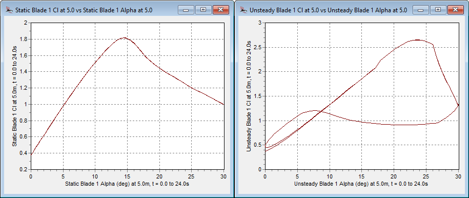
Previously, the user-specified static aerofoil coefficients, were always applied directly, without modification. However, a turbine operating in skewed/turbulent conditions, or oscillating under wave action, can experience inflow that is not steady. In such cases, unsteady flow effects, including dynamic stall, can become important.
Version 11.3 introduces two unsteady aerodynamic models: González and Minnema Pierce. Based on the semi-empirical Beddoes-Leishman model, they act to modify the static aerofoil coefficients, to account for unsteady attached flow, trailing-edge flow separation, dynamic stall, and flow reattachment. These unsteady phenomena can be characterised by rapid change, delay, and hysteresis of the aerodynamic load.
For example, the below plots show lift coefficient vs angle of attack (alpha) for the same aerofoil, undergoing oscillatory pitching motion, with (left) and without (right) unsteady aerodynamics enabled:
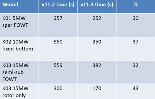
Improved performance
In version 11.3 we have optimised the turbine calculation code. In some cases, this can result in a significant reduction in the time required to run a wind turbine simulation. For example, in models containing only a turbine object, this can be as much as 40%. For a more typical FOWT model, containing a floating platform and mooring system, then a smaller reduction would be expected. To give some indicative vales, the below table shows the times taken to run the wind turbine example suite, on a single thread:
OrcaWave
Dipoles
OrcaWave models can now include dipole panels to describe structures which are thin and have water on both sides. Examples of such structures include heave plates and strakes, shown in green in these models:
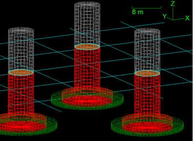
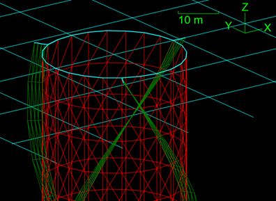
The radiation and diffraction effects of the thin structures are captured in the calculation, including a pressure discontinuity between the water on opposite sides.
Mean drift full QTFs
You can now include mean drift QTFs in a full QTF calculation, in combination with restricting the QTFs to a band of dynamic frequencies. The data look like this:
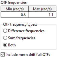
This means you can restrict the time-consuming QTF calculations in OrcaWave, and also obtain mean-drift results to be used for static analysis in OrcaFlex.
Morison element added mass and fluid inertia
In version 11.2 we introduced Morison elements to capture hydrodynamic drag loads in OrcaWave. Following requests from users, in 11.3 these are extended to include added mass and fluid inertia loads. The analogous Morison element objects in OrcaFlex have been extended in the same way, as described below.
Restarts
Restart analyses were introduced in version 11.1. Although the functionality was already quite comprehensive, some important enhancements have been made in version 11.3:
- Restart analyses were previously not allowed for models that included line feeding. That limitation has been removed in version 11.3.
- In previous releases, restart analyses could only start from the end of the parent analysis. It is now possible to restart from a specified time in the parent analysis. This latter option is known as a mid-simulation restart.
- The OrcaFlex GUI has facilities for presenting collated results for the entire restart chain, a very convenient feature. Previously this functionality was not available from the API and so users needed to collate results manually in their post-processing code, which was somewhat inconvenient. Version 11.3 extends the API to support extracting collated results.
Truss structure modelling
Lines now have an option for OrcaFlex to automatically calculate the line’s length and end orientations from the positions of the line ends. If this option is selected, then the total unstretched length of the line is set equal to the distance between end A and end B in reset state, and the z-axis of the local axes at each end will point along the straight line running from end A to end B.
This functionality could potentially have a variety of uses, but the primary motivation was for truss structures like this:
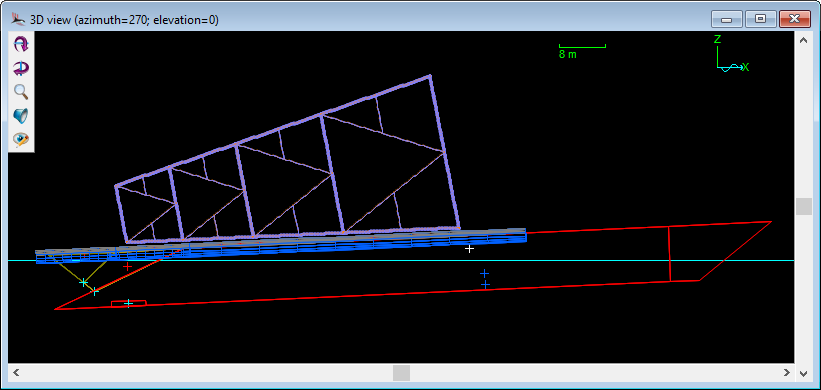
This model was developed internally to demonstrate modelling a jacket launch. Each truss member is modelled as a distinct line. When we originally developed the model, we needed to calculate and specify the unstretched line lengths and end orientations for each member. This is a very painstaking and time-consuming process. With the new functionality, the line lengths and end orientations are calculated automatically by OrcaFlex. This greatly simplifies and streamlines the model building process.
DNV ST F101 2021 code check update
The code checks feature has been updated to reflect the latest DNV ST F101 2021 edition. New data and results have been added to facilitate this.
The older DNV OS F101 results, which pertain to the 2012 edition, are still supported.
Morison element added mass and fluid inertia
Morison elements (introduced in 10.2) are composed of a collection of rigid cylinders which attract hydrodynamic loads. Morison elements can be connected to either vessels or 6D buoys, although the most typical usage is to connect them to vessels. An example of their use might be to include the influence of quadratic viscous drag on the bracing of a semi-submersible, which has been neglected as part of a linear hydrodynamic diffraction analysis.
In previous versions, Morison elements attracted drag loads, but no other loading. A number of users have requested that we also include added mass and fluid inertia effects, which we have done in this release. The input data are shown below:
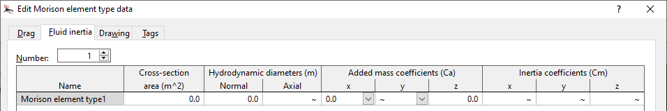 As mentioned above, we have also extended the analogous Morison element feature in OrcaWave in the same way.
Embedded Python optionally included in OrcaFlex installation
OrcaFlex has the ability to host an embedded Python interpreter to execute Python code directly from OrcaFlex. This is used by external functions, post-calculation actions, user-defined results, etc. Support for embedded Python has been part of OrcaFlex for some time now, but it has become much more mainstream with the introduction of the turbine object. The generator and pitch controllers required by turbine objects are typically implemented using Python external functions.
Installing Python is an extra task for any OrcaFlex user that wants to use Python with OrcaFlex. This task can sometimes be a little tricky, and may rely on support from your IT department. As well as installing Python, you must also install some additional Python modules.
The 11.3 installer can now (optionally) install an embedded Python distribution. This distribution is based on the embedded package available at python.org with a small number of critical third-party modules included: pip, NumPy, SymPy, PyYAML and OrcFxAPI.
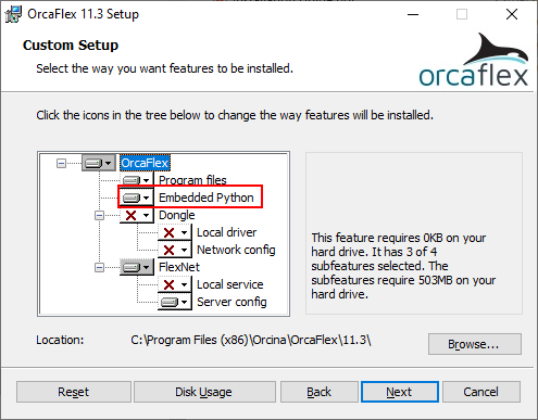
If you choose to install this embedded Python distribution whilst installing OrcaFlex, then this Python distribution will be used by OrcaFlex as its preferred embedded Python. This allows you to use Python external functions, post-calculation actions, user-defined results etc. without having to install a Python distribution separately.
The embedded Python distribution is also included in the demo version installer which means that you can install the demo version and load our turbine examples without a separate Python installation step.
Conclusion
We hope that you all find some useful and valuable improvements in OrcaFlex 11.3. And while you get to grips with it, we will start working on developments for the next release!