We are very pleased to announce the release of OrcaFlex version 11.2. The software was finalised and built on 22nd November. All clients with up-to-date MUS contracts will receive, in the week starting 29th November, an e-mail with instructions on how to download the new version.
Version 11.2 introduces much new functionality, including:
- Seabed resistance modelling
- Turbine shear centre offset
- Turbine drivetrain flexibility
- OrcaWave restart analysis, variation models and change tracking
- OrcaWave Morison elements and stochastic drag linearisation
- OrcaWave decomposed panel results
- OrcaWave body data origins
- OrcaWave connections
- Vessel inertia compensation
- Extended Wavefront .obj support
These are the most significant developments, in our opinion. As always there are more enhancements that are not listed here. All new features are fully documented in the what’s new topics:
What follows is a brief introduction to each of the new features that we consider to be of most significance.
Seabed resistance modelling
A number of enhancements have been made to the way OrcaFlex models interaction between line objects and the seabed. This interaction can be split into two separate parts: normal and tangential. The modelling of normal reaction force is unchanged and the new functionality is all contained in the modelling of the tangential resistance.
The tangential resistance is sometimes considered as two perpendicular components, which we previously referred to as the normal and axial components of the tangential resistance. There is potential for confusion in our use of the term normal here, as it clashes with the term used for the normal reaction force. And so in version 11.2 we have switched to using the terms lateral and axial for these components of tangential resistance, which also follows the prevalent convention used in published literature.
In previous versions, tangential resistance could only be modelled by Coulomb friction. In version 11.2, some new options have been added to the Coulomb friction model, and a new seabed resistance profile model has been added which can be used instead of, or in conjunction with, the Coulomb friction model.
Starting with the changes to the Coulomb friction model, these are as follows:
- A decoupled model of lateral and axial friction has been added for seabed interaction. This model does not average the lateral and axial friction coefficients and instead treats them as defining independent forces.
- An option has been added to allow seabed contact forces to be applied at the line centreline when torsion is included, rather than at the point of contact. This may be more appropriate for a line embedded in the seabed, as applying the force at the contact point might lead to unphysical twisting of the line.
These changes have been made in response to feedback from users. Both of these new features are optional and the previous Coulomb friction model is still available should you wish to use it.
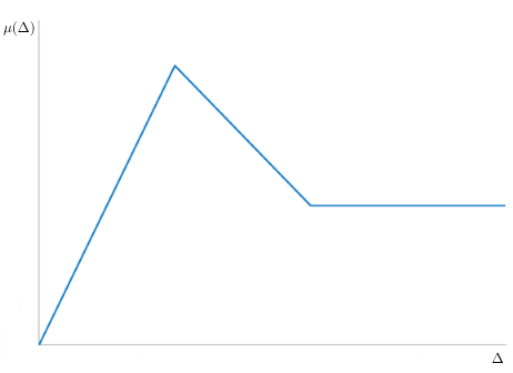
User-defined seabed tangential resistance profiles can now be added. These provide new modelling options for the interaction between the line and the seabed, and may be used for applications such as pipeline breakout or slip. A resistance profile is specified by a data table of normalised resistance (the ratio of the magnitude of the tangential force to the magnitude of the normal force) versus displacement.
A typical example is a trilinear resistance profile, in which there is an initial peak of resistance, corresponding to the force needed to break the line out of its initial (as laid) trench in the substrate, followed by a smaller, residual constant resistance representing the work done by the line in pushing the soil ahead of itself as it moves across the seabed.
For the next release of OrcaFlex we are planning to include features to model expansion and contraction of pipes due to variations in temperature and pressure. We also plan to allow a much more general slug flow and contents specification in a line. These features, together with the addition of restarts in 11.1 and the changes to seabed resistance modelling in this release, are intended to enable much improved modelling of pipeline and riser interaction with the seabed.
Turbine shear centre offset
The location of the shear centre can now be specified for the turbine blade profile. This allows the blade model to capture structural couplings which can be important for some turbine designs. In our upcoming user-group meetings we will present some comparisons with NREL’s BeamDyn to demonstrate the impact of this.
Turbine drivetrain flexibility
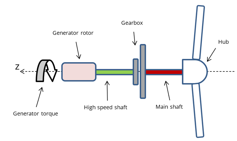
To allow for drivetrain flexibility, the turbine’s main shaft stiffness and damping can now be specified. If a finite stiffness is given, the hub can rotate, about the main shaft axis, relative to the gearbox’s main shaft output, and linear damping can be included. If stiffness is specified to be infinite, then the drivetrain has no flexibility, as was the case in previous versions.
OrcaWave restart analysis, variation models and change tracking
In 11.1 we introduced intermediate results. In 11.2 this feature has been renamed as restart analysis, and slightly enhanced. The core functionality is unchanged – you can use saved results from a previous OrcaWave analysis to perform an accelerated calculation.
The new name and workflow are designed to be as close as possible to the analogous functionality in OrcaFlex. We have introduced change tracking, just as we did in OrcaFlex.
![]()
This has the benefit of making it easy to see which data has been modified.
Finally, the concept of variation files has been brought across from OrcaFlex, also using change tracking.
OrcaWave Morison elements and stochastic drag linearisation
OrcaWave models can now include Morison elements – rigid cylinders which attract hydrodynamic drag forces. Since Morison drag is quadratic, stochastic linearisation is performed to obtain a linearised drag model which can contribute to the first-order equation of motion. Linearisation is performed for a given sea state, defined by a wave spectrum.
The linearised drag will affect results for displacement RAOs (and quantities dependent on them, such as QTFs). Drag does not affect results for load RAOs, added mass or damping. A typical application is a full QTF calculation in a situation where hydrodynamic drag has a significant effect on body motion. Drag would be included in order to improve the displacement RAOs, and hence the QTF results.
OrcaWave decomposed panel results
In response to numerous requests from users, decomposed panel results have been added to the panel results that can be accessed via the API. Panel pressure (or velocity) is decomposed into separate contributions from the diffraction potential and the components of the radiation potential.
OrcaWave body data origins
Also in response to user feedback, we have introduced new data items that allow you to specify inertia data relative to an origin of choice, e.g. the centre of mass.
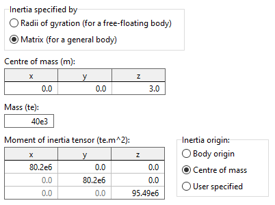
One of the most common sources of confusion encountered by users of OrcaWave has been how inertia data is specified. In previous versions these data were specified relative to the body origin. In 11.2 you can choose between the body origin, the centre of mass, or a user-specified origin.
OrcaWave connections
It is now possible to specify that a body is rigidly connected to another body. This allows you to model the separate hulls of a semisub, catamaran or similar as separate bodies. A connection affects the displacement RAOs of both bodies, and all the result quantities that depend on them, such as QTFs. The principal motivation is users performing multi-vessel OrcaFlex analyses in order to study dynamic connection loads.
Note that you cannot use this feature to divide a simple hull into parts. Each OrcaWave body must look like a standard body, i.e. a closed surface surrounded by water. We have had a couple of requests for the even more complicated case of dividing a simple hull into parts, but that would require further development.
Vessel inertia compensation
OrcaFlex models may contain floating bodies that carry a relatively large superstructure. By this general description we mean that the superstructure represents a significant proportion of the total mass and inertia of the floater. Detailed modelling of the superstructure may be a further requirement of the analysis, such as when analysing transport or installation of heavy topsides, or floating wind turbine systems.
To represent the floating body, a diffraction analysis is carried out to provide input for definition of an OrcaFlex vessel type. A typical diffraction analysis would require the total mass and inertia of both the hull and the superstructure as input.
When the diffraction analysis output is used in the OrcaFlex analysis, there is the possibility for double-counting of the superstructure inertia. The inertia is counted as part of the floater in the OrcaFlex vessel type, and that same inertia can also be explicitly represented by the OrcaFlex objects used for the detailed superstructure model.
If the superstructure is modelled explicitly in OrcaFlex, then you would need to adjust the mass and inertia of the vessel to compensate for the mass and inertia of the superstructure. We previously provided a spreadsheet to perform inertia compensation. In version 11.2 we now provide data items on the vessel data form that allow OrcaFlex to perform this task directly.
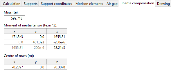
This data should be filled out with the mass and inertia of the superstructure that is modelled explicitly by other objects in your OrcaFlex model. A convenient method for obtaining this data is to make use of the OrcaFlex compound properties report.
Extended Wavefront .obj support
Previously it has been possible to use Wavefront .obj files with OrcaFlex shaded graphics to represent bodies, e.g. vessels, PLETs, etc. In 11.2 Wavefront .obj files can also be used as OrcaWave mesh files, and for OrcaFlex wire frame drawing import.
As a consequence of this development, we have changed the way we handle axis conventions for Wavefront .obj files when used as an OrcaFlex shaded drawing. OrcaFlex maintains compatibility with old files, so that if you open a binary data file prepared with an older version of OrcaFlex, the shaded drawing data will be modified to match the new handling of axis conventions. Full details can be found in the documentation.
Conclusion
Due to the delayed release of 11.1, there are fewer new features in 11.2 than there were in 11.1. In spite of this, we hope that you all find something of value in OrcaFlex 11.2. And while you get to grips with it, we will get to work on developments for the next release!