Once again, it’s that time of year at Orcina where we release a brand new version of OrcaFlex and so we are very pleased to announce the release of version 10.3. The software was finalised and built on 28th November.
A particular novelty this year is that we are now distributing the software electronically. Finally we have moved in to the 21st Century and will no longer be sending you CDs in the post! All clients with up-to-date MUS contracts should receive by e-mail instructions on how to download the new version.
Version 10.3 introduces much new functionality, including:
- A new turbine object designed for modelling of floating wind turbines. This is a composite object with dedicated models for the generator, gearbox, hub and blades.
- Quasi-dynamic mooring analysis is now possible through the addition of a comprehensive analytic catenary solver.
- User defined results which allow you to extend OrcaFlex by defining, using Python scripts, additional results.
- Object tags, a set of user defined name/value pairs associated with objects in an OrcaFlex model. Tags are intended for use by external functions, post calculation actions, user defined results, post-processing scripts etc.
- Line pre-bend data can now be visualised at the point of data input, and can be specified in a more convenient format than in previous versions.
- Friction can now be included in the line support contact model.
These are the most significant developments, in our opinion. As always there are more enhancements which are fully documented in the What’s New topic for 10.3.
What follows is a brief introduction to each of the new features that we consider to be of most significance.
Wind turbine modelling
OrcaFlex is already widely used for analysis work related to fixed foundation offshore wind turbines, e.g. installation, power cables, CPS, etc. These applications do not require modelling of the turbine. For floating wind turbines, the global system behaviour features strong coupling between the aerodynamic loading, the blade structural response, and the platform response. Because of these couplings, global analysis for such systems must model all of these aspects.
Since 2011 we have offered FASTlink, a coupling between OrcaFlex and NREL’s FAST/Aerodyn codes. OrcaFlex models the moorings and platform and FAST/Aerodyn models the tower and turbine. FASTlink couples the two codes. In fact, FASTlink has been used to couple OrcaFlex with a number of other aerodynamic codes that could take the place of FAST/Aerodyn. Coupling to an external code is rather cumbersome but was previously necessary given the lack of facilities in OrcaFlex to model turbines.
Starting with version 10.3, we have developed features to model turbines directly in OrcaFlex. This allows for a much more efficient and effective workflow. The new turbine object has the following features:
- Blade Element Momentum (BEM) model for aerodynamic loading
- Turbine blades represented by beam elements that are very similar to OrcaFlex line objects
- Blade pitch control and generator control specified by external function
- Full field wind specified by importing full field wind time histories specified in an external TurbSim .bts binary file
During the development phase, we contemplated a number of options for modelling the aerodynamic loading. A number of other codes opt to link to AeroDyn. We considered this approach but decided instead to implement a BEM model directly in the OrcaFlex code. The BEM theory that we have adopted is based closely on that used by AeroDyn v15, and much of our internal validation of the OrcaFlex BEM model is a comparison against AeroDyn.
We are continuing to work on the OrcaFlex turbine model and in future releases plan to extend it to include
- Blade / tower interaction
- Dynamic stall
- Dynamic inflow
- subsea modelling, i.e. for marine hydrokinetic devices
as well as a number of other features. If there is any functionality that you would like to see added, or you have any other feedback, then please let us know.
To give a flavour of the new functionality, the video below shows an OrcaFlex shaded graphics replay of a model of the NREL 5MW turbine on the OC3 Hywind spar.
Quasi-dynamic mooring analysis
A number of developments have been introduced in recent releases that target mooring analysis applications. The latest of these, is the support for quasi-dynamic analysis, where the mooring lines are modelled using an analytic catenary representation instead of the usual finite element representation. This typically leads to very significant reductions in analysis time.
Quasi-dynamic analysis is a long established method for mooring analysis. It is described, for instance, in the BV rule NR 493, Classification of Mooring Systems for Permanent and Mobile Offshore Units. The method is implemented by a number of codes, including ARIANE and MIMOSA.
Using an analytic catenary representation is often a valid approximation for mooring lines since their bend stiffness is small and can usually be neglected. However, representing the mooring lines using the analytic catenary equations also means that no source of line damping is included. Therefore, an effective quasi-dynamic analysis will often require an additional source of damping to account for the line damping. This can be achieved by using analytic catenary lines in conjunction with vessel other damping.
For a typical quasi-dynamic mooring analysis, because mooring line loads are calculated from analytic catenary equations, the only calculated degrees of freedom in the system are those of the vessel. This is the reason for the reductions in analysis time.
For quasi-dynamic analysis, it is usually possible to use the explicit time domain solver with a large time step (as large as possible whilst retaining accuracy). The advantage of the implicit time domain solver arises when it is used with a much longer time step than would be required with the explicit solver. When the explicit solver is stable for long time steps, it will be faster than the implicit solver at the same time steps.
In designing the new functionality we have made every effort to integrate it seamlessly with existing functionality. The intent is that you should be able to build a single model of your mooring system and easily perform frequency domain analyses, quasi-dynamic analyses and nonlinear finite element time domain analyses, all from the same base model. This allows you to select and use the most appropriate tool for each stage of your mooring analysis without having to re-build the model in different programs.
User defined results
It is now possible to set up your own user defined results. These allow you to extend OrcaFlex by defining, using Python scripts, additional results.
User defined results are, in essence, a convenience feature for post-processing. There is nothing that can be done with user defined results that could not be done with other forms of post-processing. The convenience is that user defined results can be used in exactly the same way as any pre-defined results. For example, you can plot graphs of your own user defined results in the OrcaFlex GUI. You can extract user defined results using any of the various post-processing interfaces available to OrcaFlex. And so on.
User defined results take advantage of the Python interface to OrcaFlex. The code to calculate the results is run inside the OrcaFlex process, by an embedded Python interpreter. The script has direct access to the underlying model, and typical usage pattern is for the script to first extract some pre-defined results, and then calculate the additional results as a function of those pre-defined results.
Object tags
Model objects (e.g. lines, vessels, line types, etc.) now maintain a set of name/value pairs known as tags. These tags are user-defined, and are not used at all by the built-in calculation routines within OrcaFlex. They are intended for use by external functions, post calculation actions, user defined results, post-processing scripts etc; you are, however, entirely free to decide if and how to use them.
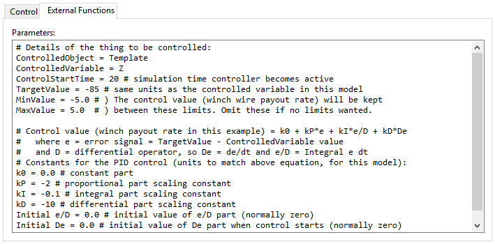
As an example, consider the PID controller from our standard set of external function examples. The external function requires a number of parameters to be specified by the user. In previous versions these were specified in a free-form text field:
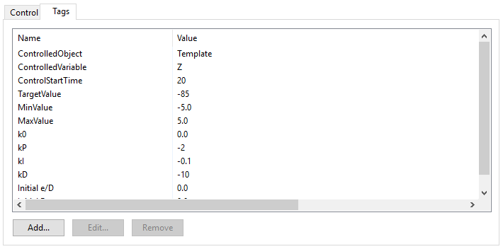
Using object tags these same parameters are specified like so:
The same information is contained in each version, but the process is much cleaner and simpler when using tags. The user experience when modifying the parameters is better when using tags. Furthermore, it is much easier to modify the tags using automation interfaces (text data file, batch script, programming interfaces, etc.)
The external function examples and user defined results examples demonstrate how tags might be used.
Simplified specification of line pre-bend data
Line pre-bend (available since version 8.5) allows you to model lines whose unstressed state is non-straight, e.g. a rigid jumper. Specifying the data for pre-bend can be tricky and so for version 10.3 we have made a couple of improvements to the usability of the feature.
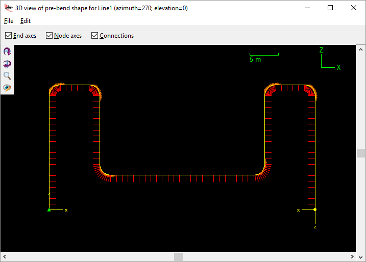
The biggest difficulty that we identified with previous versions was an inability to visualise the pre-bend shape. The data page for pre-bend data now has a button captioned view pre-bend shape which can be used to show a 3D view of the unstressed line shape and node orientations:
Multiple such view windows can be opened, for instance to show plan and elevation views simultaneously. Edits to the data are instantly reflected in any open view windows.
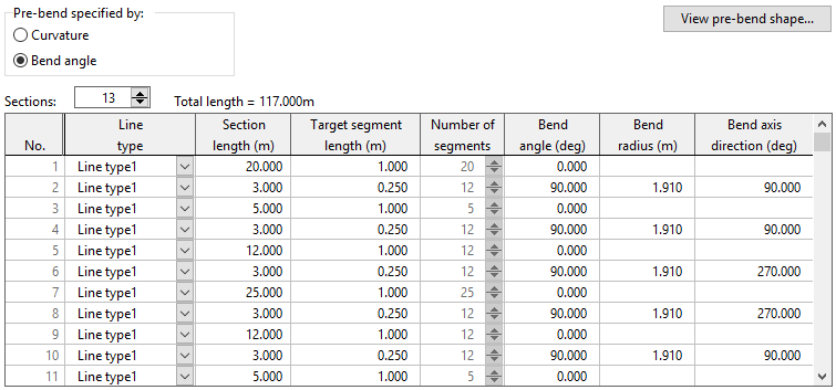
In addition to this enhancement, we have provided an alternative way to specify pre-bend data. Previously the pre-bend shape was specified by entering the x and y components of curvature. As an alternative, the pre-bend shape can now be specified by entering bend angle, bend radius (or equivalently arc length) and the angle that defines the plane of bending. For example, the above shape is specified by the following data:
Although these pre-bend developments add no new modelling capabilities, we hope that you find the user experience to be much more convenient.
Friction for line supports
In previous versions of OrcaFlex, the line support contact model did not include any friction forces. Version 10.3 adds the ability to include friction for line supports. The friction coefficients are specified on the friction coefficients data form. This data form was previously known as the solid friction coefficients data form – the name was changed to reflect the wider applicability of the form.
There isn’t a great deal to say about this development. The friction model is the same as used for seabed contact, elastic solid contact and line contact models and so should be familiar. One potential pitfall is the definition of normal and axial friction coefficients. In the OrcaFlex friction model, these directions are defined with respect to the penetrating object’s local axes. For contact between lines and the seabed or elastic solids the penetrating object is the line, and so normal and axial friction coefficients are defined relative to the line’s axis. However, for line support contact the support is the penetrating objects, which in turn means that normal and axial friction coefficients are defined relative to the support’s axis.
Conclusion
So, that’s OrcaFlex 10.3. We hope you enjoy it, and find good use for the new features. We are already busy working on the next version which you can expect to see towards the end of 2019.


