We are very pleased to announce the release of OrcaFlex version 11.0. The software was finalised and built on 28^th November. All clients with up-to-date MUS contracts should receive, by e-mail, instructions on how to download the new version.

Version 11.0 introduces much new functionality, including:

• Diffraction analysis
• Enhanced wind turbine modelling
• Wind drag loading for 6D buoys
• Enhanced wind specification
• Disturbed sea state results for vessels
• New results variables
• Hysteretic constraint stiffness
• Enhancements for 3D views
• Software licensing

These are the most significant developments, in our opinion. As always there are more enhancements that are not listed here. All new features are fully documented in the what’s new topic for 11.0.

What follows is a brief introduction to each of the new features that we consider to be of most significance.

Diffraction analysis

Starting in February 2018 we have been developing diffraction analysis capabilities for OrcaFlex. Although there is still further functionality that we intend to implement, we are now ready to release this diffraction capability. The introduction to OrcaFlex of this major new area of functionality is what prompted the major version increment to 11.

Diffraction analysis has been implemented in a separate executable, named OrcaWave. This is because we felt that it would lead to a better user experience. However, we must stress that OrcaWave is licensed as part of the OrcaFlex product. If you have a licence of OrcaFlex, then you have access to OrcaWave.

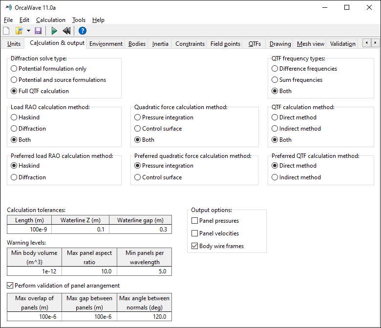
The user interface for OrcaWave is very simple compared to OrcaFlex. Everything takes place inside a single window, albeit with data and results spread across a number of pages. The screenshot below shows the calculation and output data page, and gives a flavour of OrcaWave’s capabilities.

We have made no attempt to implement any meshing functionality in OrcaWave. Instead we rely on users providing panel meshes. Perhaps at some point in the future we may add meshing, but it is not high on our priority list right now. At Orcina we have used, for example, Rhino to produce meshes and no doubt users are familiar with plenty of other meshing tools. At the moment OrcaWave can accept meshes in Wamit .gdf and Nemoh .dat format. We do expect this list of supported formats to grow in future releases. The screenshot below shows the mesh view page.

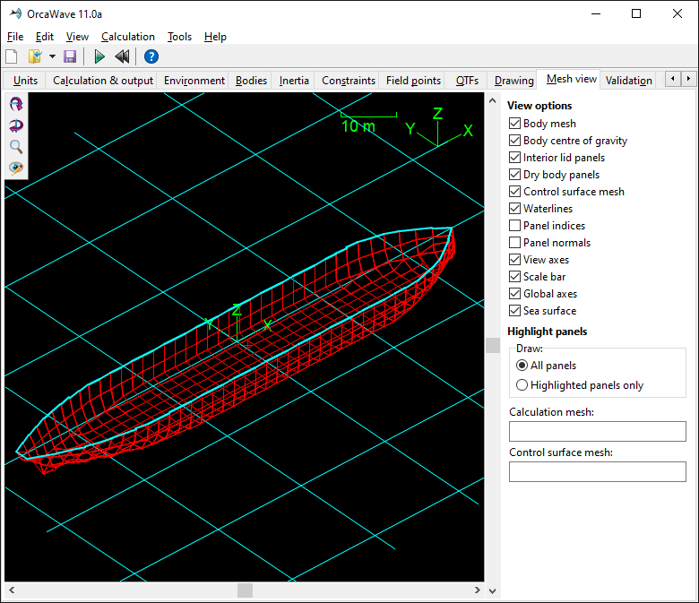
We have thought hard about the mesh visualisation functionality. The quality of diffraction analysis frequently hinges on the quality of the provided mesh. Being able to visualise that mesh aids hugely in diagnosing problems with your analysis. The view options allow you to select exactly what is displayed in the view. The highlight options allow you to identify specific panels from the mesh, and works very smoothly with the mesh validation feature of OrcaWave.

Results from the analysis are available in both graphical and tabular form. OrcaFlex is able to import hydrodynamic data from OrcaWave analyses, and because the two programs are designed to work together there is none of the uncertainty over conventions that can sometimes arise when importing hydrodynamic data.

We have validated OrcaWave by comparing its output to that of Wamit, for cases covering the entire range of functionality of OrcaWave. We have not yet had time to turn that validation exercise into a published document, but we intend to do that over the next few months.

We have merely scratched at the surface of what OrcaWave offers. Full details can be found in the program documentation.

We should once again stress that this is the first release of OrcaWave and so there is still some desirable functionality that we have not yet had time to implement. Perhaps most significantly, the program currently uses direct matrix solvers. We are aware that, for large meshes, performance can be greatly improved using iterative solvers. We will address that in the next development cycle. We are sure that users will have many other feature requests, and we look forward to receiving such feedback and prioritising future developments.

Enhanced wind turbine modelling

Last year’s release, version 10.3, introduced the turbine object designed for modelling horizontal axis wind turbines. Since 10.3 was released, we have made a number of further developments to the turbine:

• The turbine can now be associated with a tower by choosing from two tower influence models. Based on potential theory, these models allow the tower’s influence on the undisturbed wind field, due to the so-called tower dam effect, to be accounted for.
• The Øye dynamic inflow model can optionally be used when calculating the rotor aerodynamic loading. This accounts for the time that the turbine’s wake takes to adjust to a change of flow conditions.
• Blade pitch angle can now be controlled for individual blades. This feature is enabled by the new data item pitch control mode. If common pitch control mode is selected, then all blades share the same pitch angle, as was the behaviour in previous versions. If individual pitch control mode is selected then each blade has an independent pitch value. Existing external function pitch controllers will need to be adapted in order to take advantage of individual pitch control.
• Slave objects can now be connected to either the turbine hub or to a given blade at a specified arc length. Previously, slave objects were always connected to the turbine hub.
• To model structural damping on turbine blades, Rayleigh damping coefficients can now be specified.
• A number of new turbine results are available.
• A convergence monitoring start time can now be specified. Before this time, any warnings associated with the BEM method failing to converge will not be reported.

Please refer to the what’s new topic for comprehensive details of these changes.

Although not new for version 11.0, it is perhaps worth highlighting the turbine controller examples that we published when we released version 10.3d.

Wind drag loading for 6D buoys

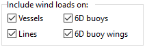
In previous versions, wind loads could be applied to vessels, 6D buoy wings and lines. Version 11.0 adds to that list by enabling wind loading on 6D buoys.

The drag load is calculated using the existing drag area and drag coefficient data. So in order to retain backwards compatibility for data files prepared with previous versions, a new option has been added on the wind page of the environment form, include wind loads on 6D buoys:

When loading old data files, this option is unchecked, so as to reproduce the original behaviour of the program. If you wish to start including wind loads on 6D buoys in existing models, you must enable this option.

For new models, this option is checked by default, and so new models are subject to wind drag loading unless you explicitly disable it.

Enhanced wind specification

Three new wind types are available:

• The ESDU wind velocity spectrum for tropical cyclone conditions.
• User defined spectrum. Analogous to the user defined wave spectrum, you provide the tabulated spectral form and then OrcaFlex generates wind components matching that spectrum. This option allows you to use an arbitrary spectral form.
• User specified components. Again this is analogous to the user specified wave components option. You enter a table listing each harmonic component from which OrcaFlex synthesise the wind time history.

Disturbed sea state results for vessels

New sea state results have been added for vessels. These include results for the disturbed wave field generated by any vessel that uses sea state RAOs.

Previously, these results could only be obtained via the workaround of attaching dummy reporting objects, such as 6D buoys, to the vessel. This workaround is functional, but it can be somewhat inconvenient. However, there are a couple of important factors that have led to us introducing disturbed sea state results for the vessel in this release:

1. You are required to decide the locations of interest before you perform your analyses
2. Adding large numbers of buoy or line objects to the model purely for reporting purposes can result in significant impact to runtime performance and output file size

The following sea state results are now available for vessels:

• Sea surface Z and sea surface clearance: undisturbed values, were available in previous versions
• Sea velocity and acceleration: undisturbed values, not available in previous versions
• Disturbed sea surface Z, disturbed sea surface clearance, disturbed sea velocity and disturbed sea acceleration: disturbed results, not available in previous versions
• Air gap: not available in previous versions

In addition to the undisturbed and disturbed sea state results, a new air gap result has been added. Because air gap is typically calculated at a large number of points on a vessel, a new air gap report has been added. A set of reporting points can be entered on the new air gap page of the vessel data form, which are then be used to generate a report of minimum air gap values for each point.

New results variables

For vessels and 6D buoys which use Morison elements, the results reporting has been significantly enhanced. Previously you could only extract results for the group of Morison elements as a whole, summed over each segment and each element. Now you can pull out per-element force results. Additionally, there are per-segment results, where the segment within an element is identified by arc length.

A number of new results variables are now available for lines:

• x relative velocity and y relative velocity, the existing result named axial relative velocity has been renamed z relative velocity
• Drag force, normal drag force, x drag force, y drag force, z drag force and lift force
• Fluid inertia force, x fluid inertia force, y fluid inertia force and z fluid inertia force
• Morison force, normal Morison force, x Morison force, y Morison force and z Morison force

All of the above are calculated from node velocity or node acceleration, or both. In previous versions of OrcaFlex velocity and acceleration results (for line nodes only) were calculated by central finite difference of the logged node positions. The decision to use finite difference rather than logging was taken to reduce the simulation file size. However, using finite difference does lead to less accuracy for the line velocity and acceleration results.

In version 11.0 you can now opt to log velocity and/or acceleration results. This choice is made on the results page of the line data form:

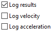
The bottom two check boxes are new to version 11.0. When checked, the program will log velocity and/or acceleration rather than using finite difference when deriving results. This change impacts all results that depend on node velocity or node acceleration, for example the new line results listed above.

Hysteretic constraint stiffness

Constraint stiffness (both translation and rotational) data can now, optionally, be treated as hysteretic. The choice between hysteretic stiffness, and elastic, is made on the variable data form:

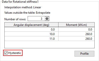
This change allows you to model friction-like phenomena. For instance, this feature could be used to model breakout friction for a turret mooring.

Reset state drawing for lines

Experienced users will recognise the image below as an OrcaFlex line drawn in reset state.

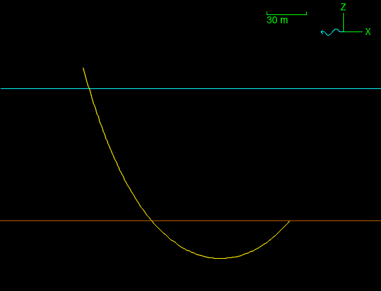
The program uses a simple algorithm to find the line shape, known as quick statics. The algorithm has been designed to be robust and efficient. As is clear to see, this algorithm makes no account for the seabed.

The image below is also an OrcaFlex line drawn in reset state, using a new feature introduced in version 11.0.

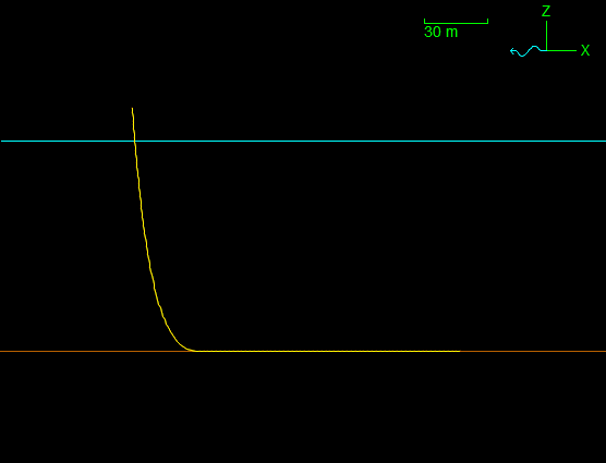
In version 10.3 we introduced an analytic catenary solver intended for performing quasi dynamic analysis. This analytic catenary solver is extremely fast, very robust, and can account for quite a wide range of line data and boundary conditions. In version 11.0, by default, OrcaFlex attempts to use the analytic catenary solver for reset state line drawing. The solver can account for flat seabeds and buoyant sections, but there are limitations. The reset drawing functionality is only used for visualisation whilst model building, and does not have any impact on calculation.

In some scenarios, it may be desirable to revert to the quick statics algorithm for reset drawing. This can be done using either a global user preference, or a setting local to individual models.

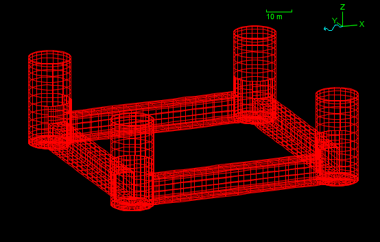
Panel mesh import for drawing

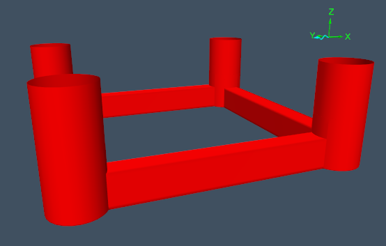
Whilst developing OrcaWave we implemented code to import panel meshes. Having written this code for OrcaWave, we have used it in OrcaFlex to import such meshes for drawing purposes. At the moment we support the same file formats as OrcaWave, namely Wamit .gdf and Nemoh .dat, but we expect this list to grow as we continue development of OrcaWave. To demonstrate, the following images were created by importing a semisub mesh from the Wamit example set.

Origin indicator marks

Another minor enhancement to the drawing routines in OrcaFlex is the introduction of origin indicator marks. These can be drawn for vessels and 6D buoys. The indicator marks show centre of gravity, centre of buoyancy, diffraction origins, etc. We illustrate this with a wire frame view showing a spar buoy object.

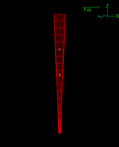
The yellow mark indicates the location of the centre of gravity, which is input data in an OrcaFlex model. The blue mark indicates the centre of buoyancy, which for a spar buoy object is calculated by OrcaFlex based on the cylinder geometry.

Slug flow drawing

Slug flow line contents can now, optionally, be drawn on the 3D view.

Software licensing

OrcaFlex now supports software licensing using FlexNet Publisher, in addition to the existing dongle-based licensing system. While the code to implement software licensing is in place in OrcaFlex, we are still developing our back-office systems. Because of this the process of obtaining and maintaining a software licence is not yet as smooth as we would wish. Bearing this in mind, if you would like to migrate some or all of your licences to the new software licensing system, please contact us.

Conclusion

So, that’s OrcaFlex 11.0. We hope you like it, and find good use for the new features. We are already busy working on the next version which you can expect to see towards the end of 2020.