We are very pleased to announce the release of OrcaFlex version 11.6. The software was finalised and built on 13th November. All clients with up-to-date MUS contracts will receive, in the next few days, an e-mail with instructions on how to download and install the new version.
Version 11.6 introduces much new functionality, including:
OrcaFlex
- Updated shaded graphics
- Frequency domain enhancements
- Improved specification for constraint stiffness & damping
- Applied loads specified by Python code
- User-specified radius for line stress results
- Nominal depth can be specified, used to evaluate wave theory and current stretching
- View filters to customise drawing on a per-view basis
- Line setup wizard can use arbitrary line results variables
- Rotate objects around an arbitrary axis using the move objects wizard
- Compound object properties can account for instantaneous positions
- References report added which lists references between objects
- More input data can now be specified in external files
- External function examples have been updated and are better documented
OrcaWave
- Memory required to perform calculations can be significantly reduced
- Body origin can now be specified by the user
- Multibody external stiffness and damping matrices
- Mesh view can now be undocked
These are the most significant developments, in our opinion. As always there are more enhancements that are not listed here. All new features are fully documented in the what’s new topics:
What follows is a brief introduction to each of the main new features.
OrcaFlex
Updated shaded graphics
OrcaFlex shaded graphics was first introduced in version 8.7, released twenty years ago in 2005. This is what it looked like:
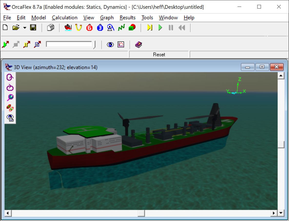
We were very proud of this at the time, but twenty years is a long time. And our shaded graphics code stood still whilst the rest of the world advanced. Looking at it in 2025 it looks a little jaded.
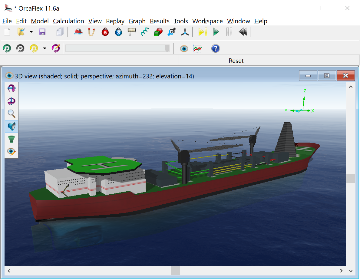
For version 11.6 we have completely re-implemented shaded graphics:
- The previous implementation was based on DirectX 9, in version 11.6 we are using DirectX 12.
- OrcaFlex now takes a physically based rendering (PBR) approach, which aims for realism by simulating the behaviour of light in the real world.
- The sea surface, seabed, and sky are drawn with advanced lighting models and allow greater customisation from the environment drawing page.
- Shadows are cast by objects in the scene according to the sun position and can add depth and realism to the rendering.
- A new parallel projection mode has been added, which matches the orthographic projection used in the wire frame mode.
- The import of 3D models has been re-implemented using the Open Asset Importer Library (Assimp). In particular this means that Wavefront .obj files are imported more faithfully. Additionally, this opens up future possibilities for OrcaFlex to import 3D models from other file formats supported by Assimp.
In version 11.6 the model above looks like this:
We are very positive about this development, and are looking forward to seeing what our imaginative and creative users do with it!
Frequency domain enhancements
A series of enhancements have been made for frequency domain analysis. Taken together these represent a significant improvement in functionality.
- After performing a frequency domain analysis at low frequency, combined linearisation solution frequencies, you can now choose whether the results are reported for the wave frequency solve or the low frequency solve. Previously the wave frequency solve was performed purely for the purpose of combined drag linearisation. Now, the results from that wave frequency solve are retained, and available for query. This development makes it easier to perform the response combinations required for mooring analysis, and we will release an example Python tool demonstrating this workflow in the near future.
- You can now connect vessels as child objects.
- Sea state disturbance RAOs are now supported, with corresponding environmental results available.
- Vessel other damping force and moment results are now available.
- Line drag force results are now available.
- Morison element drag force and Morison element segment drag force results are now available for buoys and vessels.
Improved specification for constraint stiffness & damping
In previous releases, constraint stiffness & damping was specified in a very simple form:
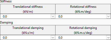
These values can be linear and nonlinear, but are isotropic, meaning that the load model is the same in all directions, e.g. motion along the x-axis has the same stiffness as motion along the y-axis. Non-isotropic models can be constructed using chains of constraints, but this can be somewhat inconvenient.
There are two new options to specify constraint stiffness & damping: specified as full 6×6 matrices or specified by Python variable data.
Specification by 6×6 matrices is hopefully self-explanatory, and so requires no further explanation.
The Python variable data option builds on the general functionality introduced in 11.5 which was used to support covered line modelling. In this context the Python variable data option allows forces and moments to be defined directly in terms of bespoke mathematical formulae.
We have illustrated this with a fun example to simulate the orbits of the planets around the Sun:
Nine 6D buoys are used to represent the Sun and the eight planets, although only the inner planets are shown here. The only relevant property of these objects is their mass. In the analysis, 36 constraints, one for each pair of celestial bodies (e.g. Uranus-Neptune gravity) are used to impose gravitational interaction between the bodies using Newton’s law of universal gravitation.
Obviously, this is not an application that we expect users to apply OrcaFlex to, but we hope that it gives a flavour of the power and flexibility of this feature. More details, including the models, are provided in the OrcaFlex documentation for constraint stiffness.
Applied loads specified by Python code
In the same vein as constraint stiffness & damping, applied loads can also now be specified using Python variable data. This allows applied forces and moments to be defined directly as mathematical functions of simulation time and (where appropriate) line arc length.
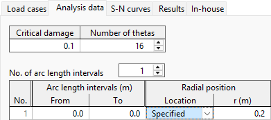
User-specified radius for line stress results
A number of line results (e.g. stress component results) depend on radial position. Previously such results were available at inner, outer and mid-wall locations. An additional option is now available, to request these results for an arbitrary radial position.
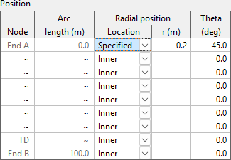
This functionality is also available for fatigue analysis.
Nominal depth can be specified, used to evaluate wave theory and current stretching
Previously, OrcaFlex used the water depth at the seabed origin when evaluating wave theory calculations and current vertical stretching. Users can now specify a nominal depth, which will be used in these calculations instead.
This enhancement makes it easier to de-couple the seabed specification from the wave theory and current stretching calculations. For 3D seabeds, the spatial origin of the 3D data was previously linked to these calculations, which was inconvenient, especially when depth varied significantly. In such cases, users sometimes had to shift the seabed data to obtain the desired environment.
View filters to customise drawing on a per-view basis
Model drawing can now be customised on a per-view basis. This is achieved by defining view filters to control the drawing properties of individual objects or object types. This includes global drawing elements such as global axes, view axes, scale bar, etc., in addition to axes and labels for individual objects. Filters use regular expression pattern matching to provide fine-grained control over the objects or object types that are matched by the filter. OrcaFlex provides tools to allow you to test your patterns. Filters are linked to each 3D view so you can control each view individually. They are saved within a workspace file but any filter can also be exported to a file for reuse. We also provide a series of view filter examples.
Line setup wizard can use arbitrary line results variables
The line setup wizard has been generalised to allow arbitrary line results variables (including user defined results) to be used as targets. Previously only a limited number of pre-determined variables could be used.
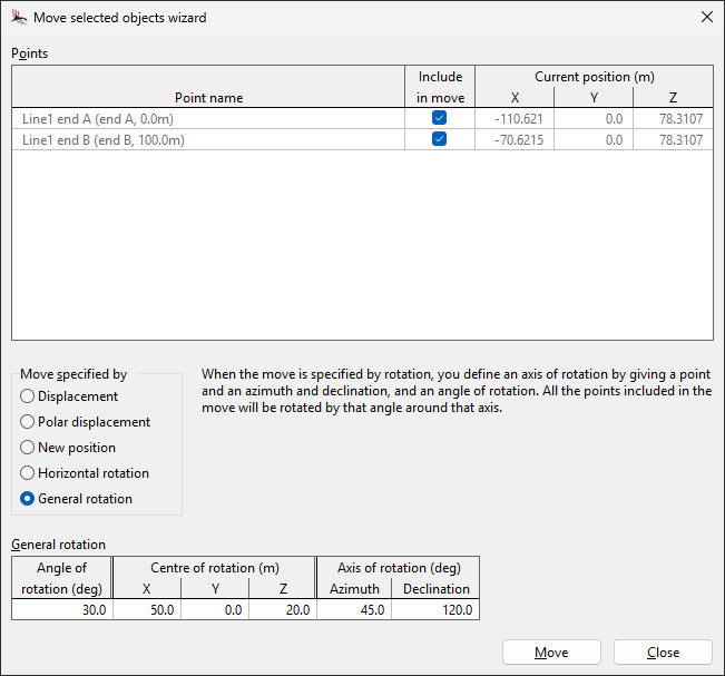
Rotate objects around an arbitrary axis using the move objects wizard
The move selected objects wizard can now rotate objects around an arbitrary axis. Previously the only rotation that was possible was rotation in the horizontal plane.
Compound object properties can account for instantaneous positions
The compound object properties report now includes wetted volume and centre of wetted volume. These properties are reported using the instantaneous object positions (in the current model state), and can account for partial submergence. However, other properties that are related to volume and buoyancy are reported assuming complete submergence, as in previous versions of OrcaFlex.
References report added which lists references between objects
A references report has been added which lists all instances where one object refers to another object. It displays, in a spreadsheet, a list of all references between objects in the model.
For simple models, it is usually obvious which objects refer to which other objects. However, for larger and more complex models, the references report can help shed light on the relationships between objects. Furthermore, if you are inspecting a model built by somebody else, it can be daunting to understand these relationships, and this new report can help.
More input data can now be specified in external files
A range of input data can be specified in an external file. Historically this was for vessel and wave time history files, and for Python code. In recent releases support has been added for this data to be specified internally, as an alternative.
There are pros and cons of both possibilities. External files are often preferable for files which are to be shared between multiple OrcaFlex files, and for external files that are very large. Defining the data internal to the OrcaFlex model file can avoid confusion and clutter in your file storage directories.
For version 11.6 we have extended the range of input data which permits both internal and external definition. This now includes:
- 3D seabed data
- Time history variable data sources (e.g. applied loads, winch payout rate, etc.)
- Wire frame drawing data and wire frame shapes, which can now be specified by an external panel mesh file
External function examples have been updated and are better documented
Previously our external function examples were installed alongside the program files, and also made available on our website. The documentation of these examples was provided in a separate PDF document. We have now integrated the external function examples into our OrcFxAPI documentation. The examples, including source code, can be downloaded directly from the OrcFxAPI documentation. The example content has been reviewed and in particular the native external function examples have been overhauled significantly. Previously these were written in C, but they are now written in C++ which makes the code significantly simpler.
OrcaWave
Memory required to perform calculations can be significantly reduced
It is possible to significantly reduce the memory required to perform a calculation using a new computation strategy data item:
- The optimised for run time strategy gives the same behaviour as previous versions of OrcaWave
- The optimised for memory strategy uses new code to perform the calculation with significantly less memory required per thread. In situations where the thread count for parallel processing is limited by the memory available on your machine, a larger thread count will be possible and the total run time of the model will be faster.
The two options give identical results; they differ only in their use of computational resources.
A separate development has also reduced the amount of memory required for some full QTF models. Models will only see a noticeable benefit if they have a very large number of panels in the free surface panelled zone, or a very large number of points in the free surface quadrature zone.
Body origin can now be specified by the user
It is now possible to choose the location of the body origin, i.e. the origin of the body coordinates system, for each body in a model. In previous versions of OrcaWave the body origin was always located on the free surface vertically above/below the mesh position. In theory, the body origin is completely arbitrary and different origins give physically equivalent results. Nevertheless it may be convenient to choose a particular origin, e.g. to simplify the preparation of input data, or to simplify the interpretation of a result that is reported in body coordinates.
Previously some, but not all, results could be reported at an origin of choice via the API after a calculation had completed. This change essentially extends that capability to all results including, for example, QTFs. However, the body origin must be decided before the OrcaWave calculation is performed.
Related to this, the centre of mass vector, required for bodies with inertia specified by matrix, has been changed. This data item is now specified in mesh coordinates \(M_\textrm{xyz}\). In previous versions it was specified in body coordinates \(B_\textrm{xyz}\).
This change was necessary because it is now possible to choose that the body origin is located at the centre of mass (i.e. the body coordinate system can no longer be used because it now depends on the centre of mass).
Multibody external stiffness and damping matrices
External stiffness and damping matrices can now be specified in a new multibody format. In previous versions of OrcaWave, external stiffness and damping matrices were always specified in a simple single-body format, i.e. as a 6×6 matrix for each individual body. The new multibody format is more general and allows for coupling between different bodies. Multibody stiffness and damping are 6N×6N matrices, where N is the number of bodies, with a block structure analogous to multibody added mass and damping matrices.
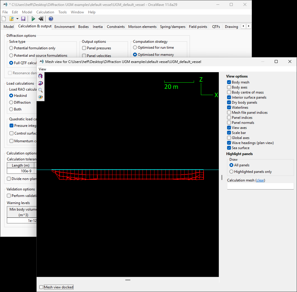
The mesh view can now be docked in the main window (as in older versions), or displayed undocked in a separate window. Displaying the mesh view undocked allows you to make changes to the input data and instantly see the impact of these changes on the model.