
|
Results: Extreme value statistics results |
|
|
Results: Extreme value statistics results |
There is often a requirement to predict the extreme responses of a system, for example to determine the likelihood of a load exceeding a critical value that may lead to failure. Such values are needed when using standards such as DNV OS F201 and API RP 2SK.
OrcaFlex can estimate extreme values for any given time domain result by analysing the simulated time history of the variable using extreme value statistical methods. You may, for instance, perform a mooring analysis in an irregular sea-state and then estimate the maximum mooring line tension for a 3-hour storm.
The statistical theory for this estimation is well-established and is described in the theory section. The procedure is essentially this:
The extreme value statistics results form is designed to lead you through this process.
When you open the extreme value statistics results form, for a selected result, you will come first to the data page, where you will select the distribution. Moving then to either of the other pages (results or diagnostic graphs) will cause OrcaFlex to carry out the estimation part of the procedure. The diagnostic graphs assist in testing the model. The results page reports the estimated statistics, e.g. the return value for the specified period, the estimation uncertainty inherent in that value etc.
For convenience, the time history result graph is reproduced on the data page. The data required for the fitting of the model are entered on this page, and are as follows.
These fall into two groups, according to the statistical method with which they are applied. For details see the extreme value statistics theory section.
Specifies whether maxima (upper tail) or minima (lower tail) are to be analysed.
These data are only required when using the Weibull and GPD distributions, which are fitted to extremes of the time history, and those extremes are selected using the peaks-over-threshold method with (optional) declustering.
The threshold controls the peaks-over-threshold method. This allows you to control the extent to which the analysis is based on only the extreme values in the data (the tail of the distribution).
The decluster period controls the declustering. This helps avoid or reduce any statistical dependence between the extreme data values used in the analysis. It can be set to one of the following:
The threshold is drawn on the time history graph, to help visualise its value relative to the extremes of the data. The number of data points that will be included in the analysis (after the threshold and declustering have been done) is also displayed. This helps with setting the threshold and decluster period.
The best value for the threshold is one that strikes a balance between a not-extreme-enough value (which will increase the number of data points fitted but may give biased fitting by allowing less extreme values to influence the fitting too much), and a too-extreme value (which will fit to only the more relevant extreme data points, but may give very wide confidence intervals if there are too few such extremes in the data).
| Note: | OrcaFlex provides a default value for threshold. This is calculated as $\mu + 3\sigma$ where $\mu$ and $\sigma$ are the mean and standard deviation, respectively, of the time history. This value is provided because OrcaFlex needs to have an initial value. However, there is no reason to believe that this initial value will be an appropriate threshold value and so we do not recommend that you use this value in your analysis. |
The following data items, found on the results page, do not affect the fitting of the statistical model. Rather, they are applied to the fitted model to obtain the reported results.
Storm duration is the return period for which the return level is reported. The length of the simulation, relative to this duration, will determine the accuracy of the estimate for the return level.
Risk factor is the probability of exceeding (or falling below, for lower tail) the estimated extreme value. For example, you may ask for the 3-hour extreme value that is exceeded with a probability of 0.01 (i.e. a risk factor of 1%).
Storm duration is defined as for the Rayleigh distribution.
The maximum likelihood fitting procedure used for these distributions allows the estimation of a confidence interval for the return level, for a specified confidence level. OrcaFlex reports this estimated confidence interval in addition to the estimated return level.
The reported return level is defined to be the level whose expected number of exceedences in the specified storm duration is one. The fitted values of the model parameters and corresponding standard errors are also reported.
| Note: | For some values of storm duration (usually small values) it might not be possible to calculate the return level. This is indicated by the value 'N/A' (meaning 'not available'). Similarly, for some combinations of storm duration and confidence level, the calculation may fail to determine the confidence limits, and again these are then denoted by 'N/A'. |
The diagnostic graphs will help you to assess the goodness-of-fit of the model, and how appropriate or not the fitted distribution is. They should be interpreted together, not in isolation, as follows.
An example of diagnostics graphs indicating a good model fit is shown below:
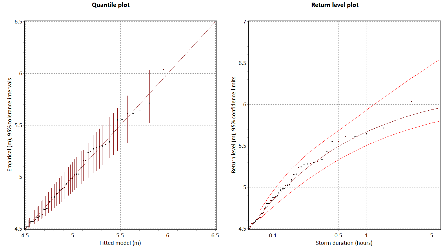
| Figure: | Diagnostics graphs for a good model fit |
If either of these graphs indicates a poor model fit, then you should reconsider the entries on the data page:
The extreme value statistics capabilities can be automated in a number of different ways.
The OrcaFlex spreadsheet post-processing facility supports analysis using the Rayleigh distribution via the Rayleigh extremes command. The Weibull and GPD distributions are not available in the current version due to the complexity of threshold selection.
The C/C++, Delphi, Python and MATLAB programming interfaces to OrcaFlex all support automation of extreme value statistics. As with all other functionality, the Python and MATLAB interfaces are the easiest to use.
The full analysis capability is available via the programming interface. That is, in contrast to the OrcaFlex spreadsheet, analysis using the Weibull and GPD distributions is available.