|
Modelling line feeding |

|
Modelling line feeding |
Line feeding is used to introduce new line, or remove existing line, during an OrcaFlex simulation. Feeding occurs at line ends, and may occur at both ends simultaneously.
As a helpful analogy, consider a flexible hose being fed into the water from a rotating drum. The drum unwinds the hose at a constant rate, so that the length of hose in the water increases linearly as time progresses. This is referred to as paying out. If the system were running in reverse, then it would remove the hose from the water and wind it back up around the drum. This is hauling in. The line that has been paid out into the water is referred to as active, and that hauled in onto the drum as inactive.
Line feeding in OrcaFlex is analogous to this flexible hose system, in that it permits the amount of active line to vary during a simulation, up to a maximum length. Where line feeding departs from the analogy is in the properties of the inactive line, which plays no part in the model whatsoever and effectively does not exist for the purposes of simulation. The inactive line is, for instance, massless – unlike the hose on the drum.
Following the above analogy, we introduce a distinction between the full line and the active line.
The full line is the 'usual' OrcaFlex line, defined by the section lengths and properties specified on the structure page of the line data form. Depending upon the specific details of the model, the full line may well represent the whole of the real physical line, including those parts of the line that are not currently deployed. In our flexible hose analogy, the full line corresponds to the entire hose, both the portion that is deployed in the water and that which is wound around the drum.
The active line is, at any time, the instantaneous part of the full line which is included in the simulation. At the start of the simulation, this is defined by the initial arc length data of the feeding line ends; as the simulation progresses, the active line may grow or shrink as line is paid out or hauled in. The active line is what OrcaFlex shows on the 3D view.
The inactive line is simply the remainder of the full line which is not active. It may be at one or both ends of the full line; if all the line has been paid out, then there will be no inactive line at all. At this point, any attempt to pay out further line will fail, and the simulation will terminate with an error message.
The full line is discretised into a number of nodes, according to its segmentation structure data, with each node being assigned a nominal reference arc length on the full line. The corresponding segment lengths are referred to as the reference unstretched lengths. These values remains unchanged throughout the simulation, so are convenient for defining fixed points and lengths on the full line.
Active line segments are continually growing and shrinking (in both size and number) as line is paid out or hauled in, meaning that the arc length of a given node, measured from end A of the full line, can vary over the course of a simulation. We refer to this as the actual arc length of the node.
Another obvious reference point is end A of the active line: the arc length of a node measured from this point is called the active arc length. So, while the node at end A of the active line has actual arc length corresponding to its position on the full line, its active arc length is always zero.
All of these arc length values are reported by OrcaFlex as position results.
The ends of the line are referred to as end A and end B for both the full line and the active line. Where this has the potential to cause confusion, it will be made explicit to which line we are referring (e.g. "full line end A", or "active line end A"). Otherwise, the meaning should be clear from the context. The reason for using the same labels in both cases is that this terminology is widely ingrained throughout OrcaFlex, sometimes naturally fitting the definition of the full line, and sometimes better suited to the active one. For instance, the end connection stiffness data on the line data form naturally apply to the active line ends, but it makes more sense to place attachments by referencing a fixed arc length relative to one end of the full line.
A given segment of the active line may be shorter (or, rarely, slightly longer) than the corresponding segment on the full line, as line is paid out or hauled in. This means that nodes are not always in the same position on the full line, which makes node results difficult to interpret: to minimise this difficulty, only the end node (and, if smooth growth is enabled, its immediate neighbour) on the active line is allowed to deviate from its reference arc length. All other nodes on the active line remain at their reference arc lengths. See below for details of the growth model.
As a simple illustration, consider a 100 m long, single-section, full line of 10 segments. It has 11 nodes at reference arc lengths of 0, 10, 20, $\ldots$ 100 m, and these arc lengths will remain associated with the corresponding nodes, regardless of the state of the active line, at all times. We can specify that just over half of the full, 100 m long, line is initially hauled in (i.e. inactive) by setting an initial arc length for end A of 55 m, and that for end B as '~'. The active line then initially spans the reference arc length range of 55–100 m on the full line and the inactive line spans the remainder, 0–55 m.
The nodes with reference arc lengths of 0 m, 10 m, 20 m, 30 m and 40 m are inactive; the node with reference arc length 50 m is the active line end node at an actual arc length of 55m; and the nodes with reference arc lengths of 60 m, 70 m, 80 m, 90 m and 100 m are active and at at their reference positions (i.e. their actual arc lengths correspond to their reference arc lengths). The initial active line therefore has five segments: the first is 5 m long, the other four are each 10 m long.

| Figure: | Full line and initial active line |
If we apply a constant positive payout rate of 0.2 m/s at end A, we will (neglecting any ramping) pay out 48 m of line over a duration of 240 s, corresponding to end A of the active line moving from actual arc length 55 m at the start of the simulation, to actual arc length 7 m at the end. At this point, all the nodes will be active and (if smooth growth is disabled) will be at actual arc lengths of 7 m, 10 m, 20 m, 30 m, $\ldots$ 100 m (if smooth growth is enabled, then the pattern will be marginally more complicated).

| Figure: | Full line and subsequent active line |
If we continue to pay out line, we must be aware that at this point we have only a further 7 m of inactive line available. After this, end A of the active line will coincide with end A of the full line. This is its ultimate extent; it is not possible to pay out any further, because there is no inactive line remaining.
This perspective views the full line as a fixed reference, and feeding as the motion of the active line ends along its length. It is helpful to adopt this viewpoint as a way of visualising the associated terminology. Physically, of course, the two ends of the active line correspond to well-defined points in space – as seen in the 3D view – and feeding can instead be thought of as the movement of line through these line ends. Each active line end may be free, fixed, anchored or connected as a child to some other object in the usual fashion: if the line ends are fixed, for instance, the amount of line hanging between them - the active line - increases or decreases according to the payout rate.
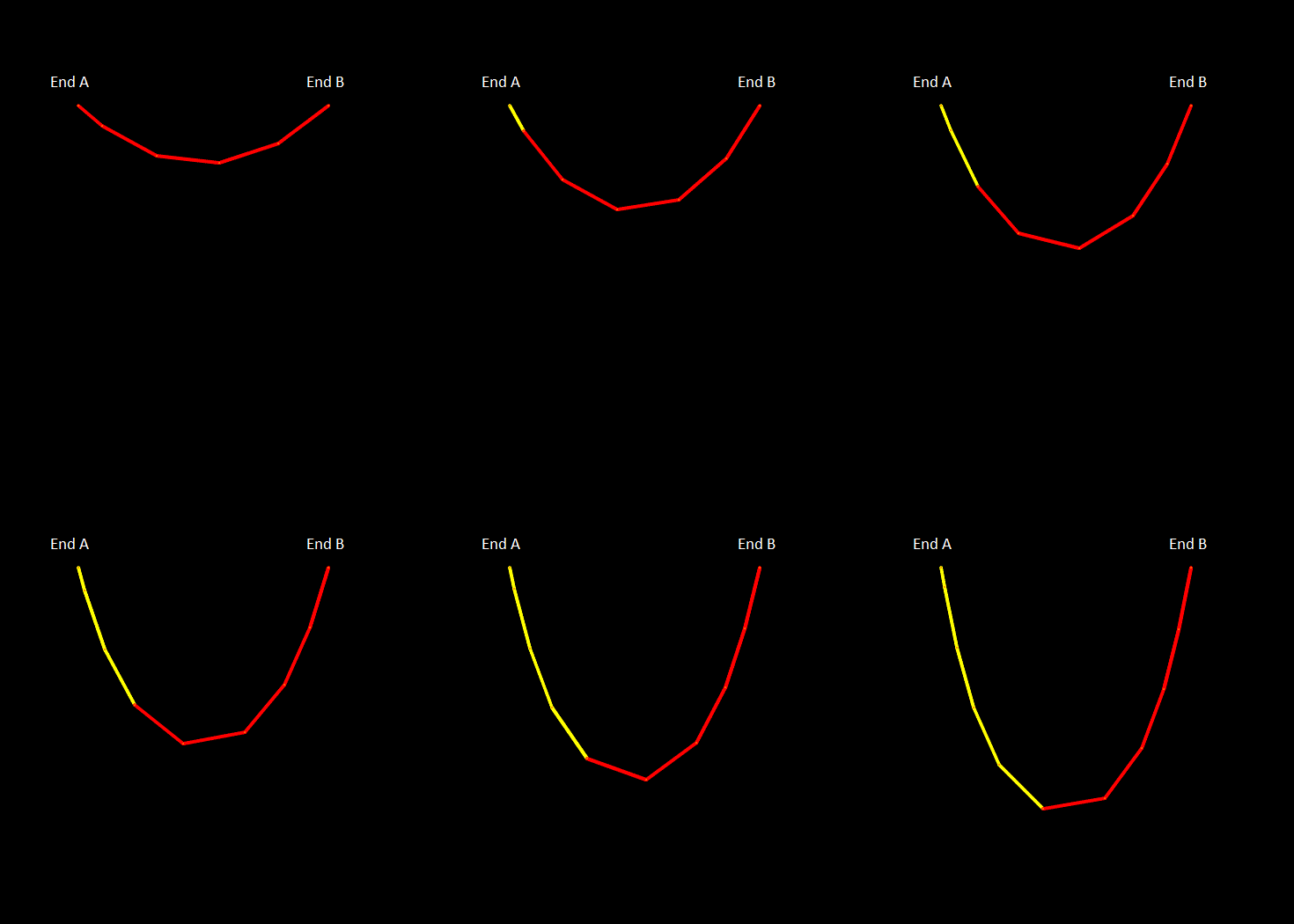
The following figure shows the evolution of this example on an OrcaFlex wire frame 3D view. Initially, the active line is drawn in red; as line is paid out, line which has been introduced (and was previously inactive) is drawn in yellow. At any point in time, the active line consists of the total length of red (initially active) and yellow (subsequently paid out) line. Remember that it is the active line which is drawn on the 3D view. In this example the (active) line ends are fixed so, as line is paid out at end A, it effectively moves from the inactive pool through the immobile end A and into the active line, and the line hanging between the ends lengthens correspondingly.

| Figure: | Line feeding, active line |
We describe the growth model here for the case of paying out. The process is, essentially, reversed when hauling in.
On paying out line, the existing segments close to the line end are grown to a point at which an inactive node needs to be made active and introduced into the active line. At this point, the new active node is placed at an arc length, relative to the feeding end, calculated as the product of the shortest viable segment factor, $r$, and the reference unstretched segment length, $l_0$.
How the segments are grown depends on whether smooth growth is enabled.
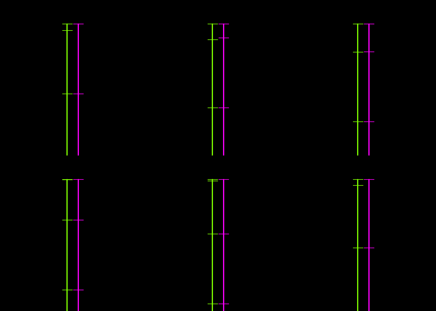
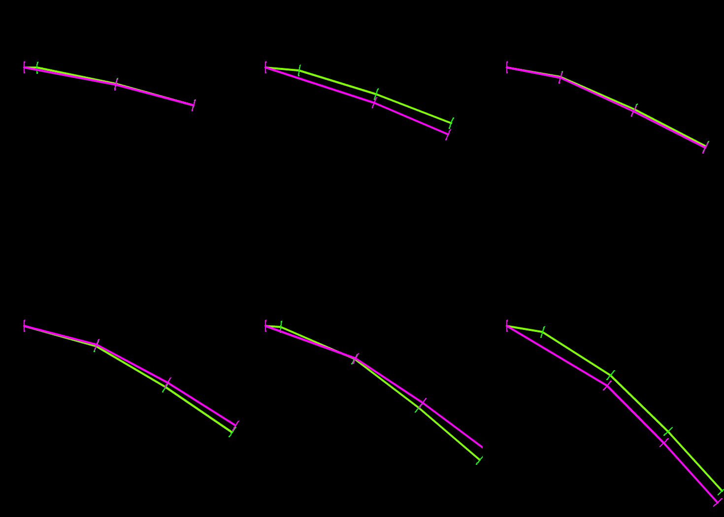
The following figures illustrate the differences between the two growth models. The left-hand figure shows the smooth-growth-enabled nodes (green line) accelerating from zero up to the full payout rate, while without smooth growth (purple line) the nodes enter the line at the full payout rate. The right-hand figure shows how disabling smooth growth can introduce noise which is avoided when smooth growth is enabled.


| Figures: | Smooth growth enabled and disabled |
The growth model is adapted in the following special cases:
The dynamic introduction of new nodes into the simulation presents a modelling challenge. A new node cannot be introduced exactly coincident with the line end, i.e. with a shortest viable segment factor of zero. In such a case, the first segment's length would be zero and, as a result, its stiffness infinite. Unfortunately, it is impossible to introduce a new node at a finite distance from the line end and for the line to remain in dynamic equilibrium in both tension and bending simultaneously. This means that the line enters a transitional regime after the introduction of the new node, whilst it adapts to the new discretisation. This can manifest itself as noisy/spiky time histories or, in extreme cases, oscillations visible in the model view. In general, as the shortest viable segment factor is increased, this noise will be exacerbated. Conversely, as the shortest viable segment factor is reduced towards zero, the segment's stiffness will approach the infinite limit and the solver will require increasingly shorter time steps to converge.
In some cases, these issues will not be present and the default control parameters will be sufficient. However, there are some prototypical cases in which these issues are expected to be important and a change to the control parameters will be required :
Another issue that can introduce noise is a discontinuous change in the payout rate. It is for this reason that OrcaFlex defaults to ramping the payout rate from zero during build-up. Occasionally, it may be desirable to suppress the ramp – such as when the build-up has already been accounted for in a variable payout rate profile – but be aware that this could potentially introduce undesirable noise in some cases.
The following features are currently incompatible with line feeding:
In addition, line feeding can currently only be used with the implicit time domain dynamics solution method.
| Note: | Rayleigh damping is compatible with line feeding but is not applied to any line segment whose unstretched length is actively varying. This is because the Rayleigh damping tends to work against the feeding and can cause the simulation to become unstable. Rayleigh damping will be applied to all line segments once they are fully grown to their reference unstretched lengths. |