Fatigue analysis: Load cases data for spectral analysis

Simulation file name

The name of the simulation file which represents the load case, either the full path or a relative path.

Line name

The name of the line, in the load case simulation file, to be analysed.

Note:

The line name will usually be the same in all load cases (though this is not necessary). The named lines in the various load cases must, of course, all represent the same physical line and use the same discretisation in the areas being analysed.

Exposure time

The total time the system is exposed to this load case.

Spectral form, spectral parameters (response RAOs only)

For response RAO spectral analysis, the simulation file name specifies a time domain response calculation or a frequency domain simulation file, from which response RAOs are derived. The spectral fatigue calculation then proceeds by combining these response RAOs with a wave spectrum to produce power spectral density (PSD) functions. This wave spectrum is of the chosen spectral form, which can be one of JONSWAP, ISSC, Ochi-Hubble or Torsethaugen.

The spectral parameters for the chosen spectral form are specified as follows:

JONSWAP spectral parameters can be automatic, partially specified or fully specified, determining exactly how the spectral parameters for each load case are to be defined. For example, if automatic is selected then you define $\Hs$ and $\Tz$; the other JONSWAP parameters are calculated automatically and their values reported.
For ISSC you must define $\Hs$ and $\Tz$ for each load case. You can also specify $\fm$ or $\Tp$ but, since $\Tz$, $\Tp$ and $\fm$ are tied together, setting any one of them changes the other two to match. There is no choice of how to set spectral parameters in this case.
Ochi-Hubble spectral parameters are either automatic or specified. If you select automatic, OrcaFlex calculates the parameters of the most probable spectrum, based on the overall significant wave height $\Hs$ that you have given. If you select specified you must specify all six parameters, from which OrcaFlex derives and displays the corresponding overall $\Hs$ and $\Tz$ values.
For Torsethaugen you must define $\Hs$ and $\Tp$ for each load case. You can also specify $\fm$ but since $\Tp$ and $\fm$ are tied together then setting either one changes the other to match. There is no choice of how to set spectral parameters in this case.

Setting up load cases for response RAO spectral analysis

When performing a fatigue analysis you will typically have a wave scatter table describing the relative probability of storm occurrence. This determines a number of wave classes, e.g. storms defined by $\Hs, \Tz$ pairs.

The load cases data should be set up to match load cases to wave classes. For example, suppose that you were working with the following (truncated) wave scatter table:

	4-5			9	3
	3-4		6	18	6
$\Hs$	2-3		22	132	117
	1-2	3	57	201	249
	0-1	15	48	69	45
		4-5	5-6	6-7	7-8
			$\Tz$

The values in the table represent joint probabilities in parts per thousand, so a value of 201 represents a probability of 0.201.

This wave scatter table gives 16 wave classes and so the fatigue analysis data in OrcaFlex would be set up with 16 corresponding load cases with appropriate pairs of $\Hs$ and $\Tz$ values.

Simulation files for response RAO spectral analysis load cases

The load case simulation file must support the calculation of response RAOs. The spectral fatigue analysis combines these calculated RAOs with the load case wave spectra (i.e. the $\Hs, \Tz$ pairs) to determine fatigue damage estimates for the load case. To support the calculation of response RAOs the load case simulation file must be one of the following:

a time domain simulation using a single wave train of type response calculation
a frequency domain simulation, solved at wave frequency solution frequencies, using a single random wave

With the exception of the wave type data (discussed below), the simulation file should model all aspects of the system and environment that define the load case. For example, you should specify vessel offset, current profile and direction, wave direction etc.

Choice of wave type data for response RAO spectral analysis simulation files

For time domain simulation files, the spectral response analysis method used to calculate the response RAOs naturally captures system nonlinearities such as hydrodynamic drag. For these nonlinear effects to be well-modelled, the choice of $\Hs$ for the response calculation wave is important.

Essentially, the RAOs can be considered as being dependent on wave height. How significant this dependence is will vary from case to case. Certain systems are dominated by linear physical effects, in which case the RAOs may well be independent of wave height. We recommend sensitivity studies to determine the significance of this effect.

In the example above, we might find that the system has significant nonlinearities and so choose to run a response calculation simulation for each row of the wave scatter table. This would give 5 simulation files for $\Hs$ ranges 0-1, 1-2, 2-3, 3-4 and 4-5. There are 4 wave classes corresponding to the 0-1 $\Hs$ range. The load case corresponding to each of these wave classes would then be represented by the same simulation file. The other $\Hs$ ranges are dealt with similarly and so the load cases table would look as below:

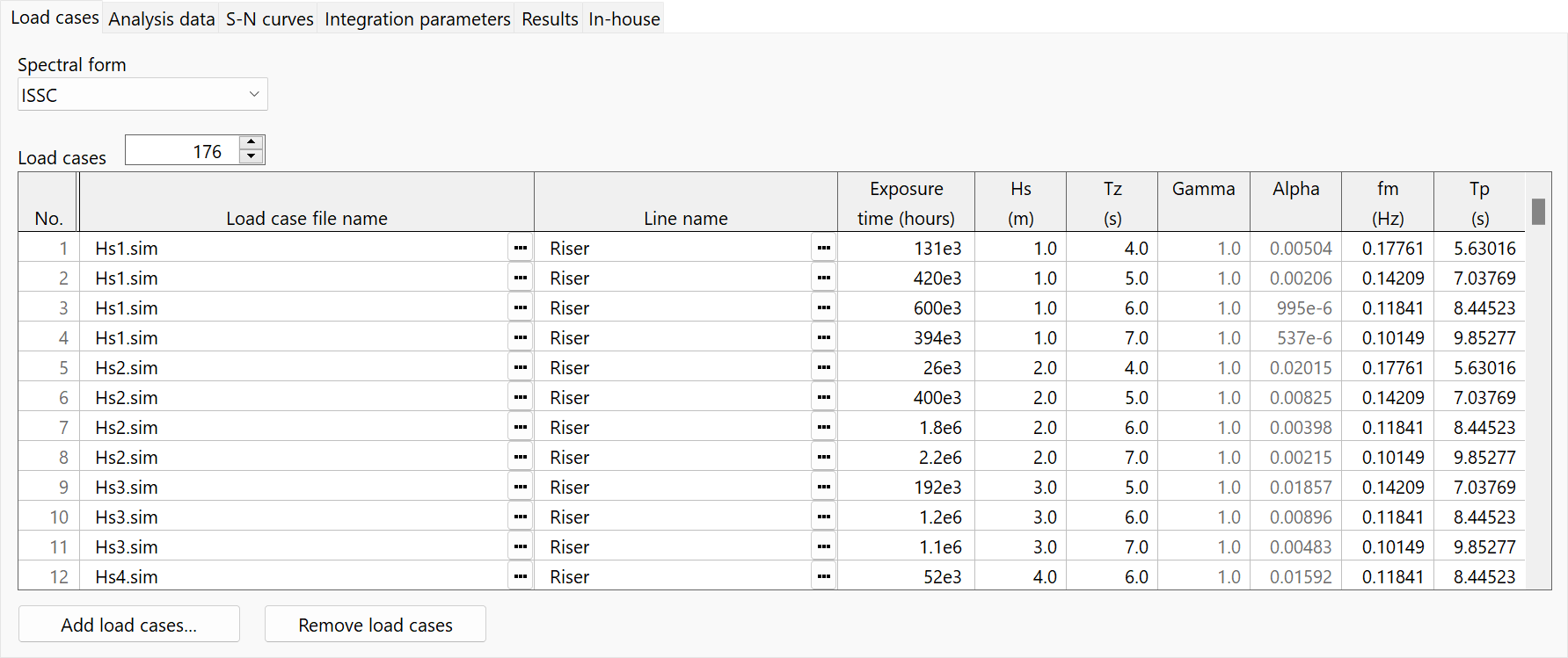
Figure:

Example load cases table

If the nonlinearities in the system are not so significant, then you may be able to obtain sufficiently accurate results with fewer simulation files, reducing the overall simulation time required. For example, the Hs1, Hs2 and Hs3 simulations could be combined into a single Hs2 simulation etc. Again, the accuracy of such a simplification should be tested with sensitivity studies.

For frequency domain simulation files, the system nonlinearities have been linearised. The process of linearisation again results in the response RAO being dependent on the wave height and, in this case, the other wave type data. Analogous to the time domain case, multiple load cases can be associated with a single simulation file and the number of simulation files needed to accurately represent all the load cases will depend on how significant the nonlinearities are. Sensitivity studies are recommended to confirm that the wave type data in the simulation file well represents all the associated load cases. In the most accurate (but least efficient) scenario, there is a unique frequency domain simulation file for each load case, and for each one the wave type data are consistent with the case's spectral parameters. Here, the linearisation is bespoke for each load case, and the frequency domain spectral analysis is equivalent to conducting a response RAO spectral analysis.

Response calculation simulation duration

The other decision to make is over the length of the response calculation simulations. You need to simulate for long enough to get accurate results. As for the issue of $\Hs$ discussed above we would recommend using sensitivity studies to determine how long is required.