We are very pleased to announce the 2014 major release of OrcaFlex, version 9.8. The software was finalised and built on 28th October. The next step is for us to prepare the installation program, and then dispatch the software. All clients with up-to-date MUS contracts should receive the new version early in November.
Version 9.8 introduces a variety of new functionality, including:
- Supports, for modelling S-lay pipe supports, and more.
- Variable slamming and added mass.
- Wave calculation optimisations to reduce simulation runtime for irregular wave cases.
- Line contact modelling improvements.
- 3DOF calculated vessels can be used with the implicit solver.
These are the most significant developments. As always there are a great many more enhancements which are documented in the What’s New topic for 9.8.
What follows is a brief introduction to each of the new features that we consider to be of most significance.
Supports
The major new development in version 9.8 is known as Supports. It is yet another contact model. The feature has been quite some time in the making and was developed originally to meet the needs of pipelay modelling, specifically S-lay. The new functionality is a contact model that has been designed to enable efficient modelling of pipelay rollers. However, this contact model can be used to model more than just pipelay rollers which is why we have chosen a rather non-specific name for the feature.
Pipelay applications using supports
It has long been possible to model S-lay with OrcaFlex, although it has never been convenient to do so. The main headache was always the modelling of the contact between lay pipe and supporting rollers. Over the years we, and our users, have come up with many different ways to model the contact, none of which has been particularly satisfactory. So the prime motivation for the new development was to make the modelling of this contact more efficient and more robust, and to make the model building simpler.
Model building is performed in two distinct steps. Firstly support types are defined. These specify the geometry and stiffness of a support. A support is composed of one or more cylinders. For instance, a V shaped support is defined like this:
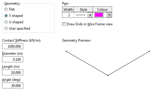
As shown in the above screenshot, a number of geometry options are available. The Flat, V shaped and U shaped options are intended to make it easy to model common S-lay roller types, and the User specified option gives you extra generality to model more complex or unusual geometries.
The second modelling step is to specify where the supports are located in the model. Supports are rigidly attached either to Vessels or 6D Buoys. Two methods to specify the geometry of the supports arrangement are provided:
- The simple geometry specification provides a quick way to set up a simple stinger model, with the supports positioned along a user-specified support path.
- The explicit geometry specification provides a method for the generation of detailed support models in arbitrary arrangements where the positions and orientations of individual supports are explicitly defined with respect to user-specified coordinate systems.
For example, the data specification for the explicit geometry specification looks like this:
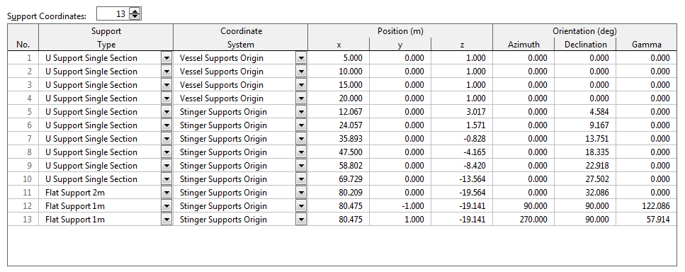
Note that the supports are specified relative to a coordinate system that, in turn, is specified relative to the vessel’s own coordinate system. This may, initially, seem unduly complex. However, the additional complexity allows you to move and rotate groups of supports. The exemplar for this is a model containing some supports attached to the deck, and other supports attached to the stinger. By defining separate deck and stinger coordinate systems we are able to, for instance, rotate the stinger about its hinge without moving the on deck supports.
The resulting model appears can be seen in the 3D View screenshot below:
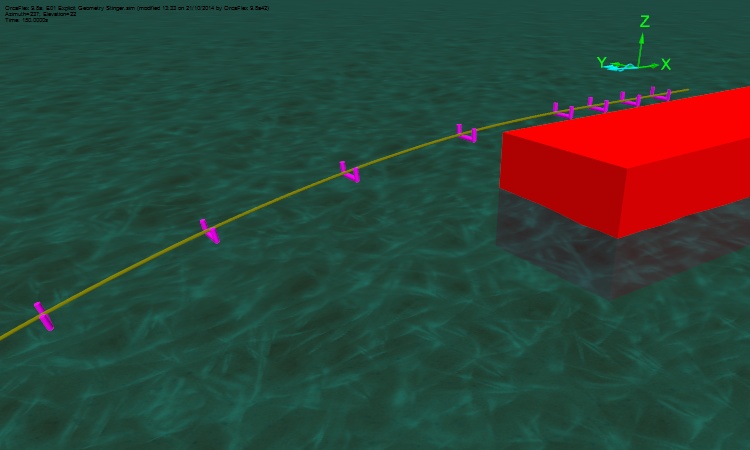
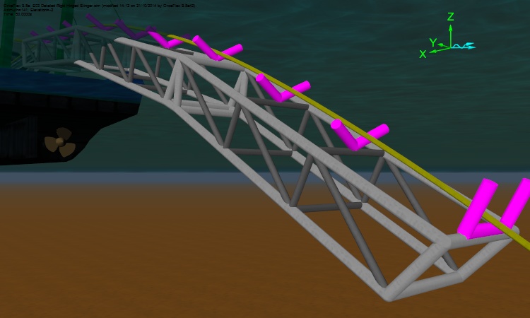
This is quite a simple model of a rigid stinger. Much more complex models can be built with ease. As mentioned above, supports can be connected to 6D Buoys as well as to Vessels. This allows us to create roller boxes that can pivot, hinged stingers, articulated stingers, and so on. The next screenshot is of a rigid hinged stinger, and is taken from our newly updated example suite.
As well allowing for much simpler model building, the new supports contact model brings other benefits. Most importantly the new contact model is very robust. Each contact cylinder has a preferred side, i.e. above the support rather than below it. This leads to very reliable and efficient statics convergence, with no need for “helper” objects to guide the line to the preferred side of the support.
The supports contact model is based on the same underlying algorithm as the line contact model. The supported lines are splined and this means that the contact point can move smoothly in the axial directions of the supported lines during dynamics. Unlike some line contact modelling scenarios, there is no requirement for torsion to be modelled in the supported lines. This means that convergence in statics is, as a general rule, quick and reliable.
The new supports functionality complements the existing capabilities of the program that are applicable to S-lay. For instance the pipelay code checks functionality, the ability to model pipe-in-pipe and piggbyback pipes, etc.
Non-pipelay applications of supports
As mentioned above, the new supports feature can be used for applications other than S-lay. The key aspect of the feature that sets it apart from the other contact models in the program is the concept of a preferred side for the supported lines. This can remove the need for “helper” objects and so greatly simplify the model building and make convergence more robust. In our 2014 season of User Group Meetings we present a number of models that benefit from the new supports contact model.
The video below shows a mid-water arch model with the guttering built using U-shaped supports. The model is quick and easy to build, and the convergence in statics is very robust. The video shows OrcaFlex performing the static analysis and shows how quick the analysis is.
The next video demonstrates a half-moon lift. Before the existence of the supports contact model, statics convergence would have presented quite a challenge. The preferred side feature of the supports contact model means that statics convergence is simple. Again, the video captures OrcaFlex performing the analysis and again it is very quick. Blink and you may miss it!
We are confident that there are many more applications that will benefit from the new supports contact model and look forward to learning from our users as they explore the new capability.
We at Orcina are all very excited by the possibilities opened up by this new feature. We hope that you the users will find the new functionality to be as useful as we believe it to be.
Variable slamming and added mass
In version 9.5 we added slam force modelling for 6D Buoys. This modelling was based on the user providing slam coefficients for water entry and water exit, Cs and Ce. These coefficients were constant. As an alternative to constant coefficients, water entry and water exit forces on 6D Buoys can now be calculated using variable slam force data that varies with submergence.
The variable slam data model follows the rate of change of added mass formulation given in DNV Recommended Practice (RP-H103, RP-C205) and it allows slamming and water exit forces to be modelled for buoys that are fully submerged but near the surface, as well as for surface-piercing buoys.
In addition to allowing slamming and and water exit forces to be variable with submergence, the program now allows 6D Buoy added mass coefficients that vary with submergence.
The new development is intended to make it possible to model water entry and exit loading more accurately. In the future we intend to allow the same hydrodynamic loading models to be applied to line objects.
Wave calculation optimisations
A critical aspect of any simulation tool like OrcaFlex is its runtime efficiency. That is, how long it takes to perform simulations. Whilst we think that OrcaFlex is already very efficient, we are always on the lookout for ways to make it even faster.
One area where there has been potential for improvement, at least in terms of efficiency, is in the calculation of wave loads for irregular seas. An irregular sea in OrcaFlex is modelled as a linear superposition of linear components. Evaluating wave kinematics (particle velocity and acceleration) involves expensive trigonometric and hyperbolic operations. Since these operations are performed for each wave component, models with large numbers of wave components can take a long time to run.
In previous versions of OrcaFlex, the wave kinematics were evaluated exactly. The kinematics were computed for each rigid body (e.g. node or buoy), at every time step. For a model whose calculation is dominated by the nodes – the usual case – a general rule of thumb is that when there are 200 wave components, half of the computational effort is spent evaluating wave kinematics. When there are 400 wave components, 2/3 of the computational effort is spent evaluating wave components, and so on. So, there is clearly an opportunity to improve efficiency if suitably accurate optimisations can be found, and version 9.8 introduces some such optimisations. The extent to which these optimisations give efficiency gains varies from model to model.
Wave Kinematics Cutoff Depth
The strength of wave kinematics decays with depth. In very deep water, it is quite possible that the majority of nodes in a model experience negligible loading due to waves. Version 9.8 now allows you to specify a cutoff depth below which wave kinematics are not calculated and are taken to be zero. For deep water cases this is the simplest and most effective way to increase efficiency.
Interpolation in time
The new version allows you to specify a time interval for wave kinematics calculations. This allows you to decouple the update frequency for wave kinematics calculations from the time integration time step. For instance, there may be structural reasons for using a short integration time step, but the wave loading varies more slowly. The program uses linear interpolation to calculate wave kinematics for time integration time steps that fall in between the wave calculation update steps.
Interpolation in space
One huge opportunity for optimisation is to evaluate the wave kinematics at fixed points in space. So long as we always evaluate the wave kinematics at fixed points, we we are able to use standard trigonometric identities to replace expensive trigonometric operations with simple multiplication and addition operations. Version 9.8 offers a couple of ways to take advantage.
One option is simply to neglect the motion of the nodes during the simulation. The kinematics are calculated assuming each node remains at its static position. This assumption could be reasonable for lines attached to fixed structures, or for low wave height bins in a fatigue analysis.
For models where using the static position is not tenable, the program offers an alternative. Instead of evaluating the wave kinematics at the instantaneous position of each node, the wave kinematics are evaluated on a spatial grid, whose spacing is determined by the user. Then, the wave kinematics for each node are calculated by linear interpolation over the grid. The program uses a grid of infinite extent, but only calculates kinematics at the grid points as needed. This adaptive approach allows the the program to be flexible and yet retain efficiency.
Sensitivity
Although the efficiency gains offered by these new developments are enticing, you must always take great care that you don’t sacrifice accuracy for the sake of reduced simulation run time. It is always advisable to perform some sensitivity studies to demonstrate that the approximations used do not unduly influence the results of interest.
Line contact modelling improvements
.
Penetrator discretisation
Since releasing the line contact feature two years ago, we have become aware of a very specific modelling issue when the line contact penetrators and the spline have the same, or very similar, diameters. An example of this is a centralised pipe, where the centralisers are in an interference fit with the outer pipe.
The program calculates penetration for line contact by calculating the closest approach of the penetrator to the splined line, and then accounting for the contact diameters of the two lines. The reaction force is applied in the direction defined by the line that passes through the two points of closest approach. Consider the case represented by the following diagram:
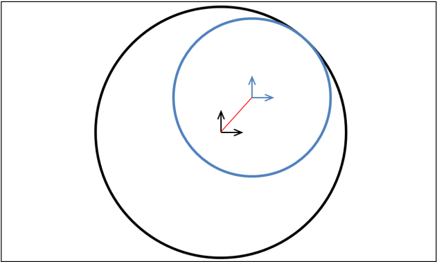
The blue line is inside the black line, and the contact diameters are quite different. When the inside line’s contact surface is just touching the outer line’s contact surface, the two centres are far apart and the direction of the line between these centre points is well-defined.
Now consider a case where the contact diameters are very similar.
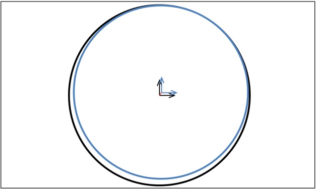
When the two lines are in contact, their centres are almost on top of each other. The direction is defined, but small perturbations in position of either line lead to large changes in direction. When the centres are exactly coincident this direction is ill-defined and the contact force model is singular.
In the case where the penetrating line and splined line have the same diameter, the singularity in the force model can lead to noisy or unstable simulations. Even if the diameters are close but not exactly the same, the force model is near-singular which can cause instability.
A new feature, penetrator discretisation, has been introduced to tackle this issue. By discretising the original penetrator into multiple smaller penetrators, placed around the original contact surface, the contact can be modelled without singularity.
The new functionality asks the user to specify how many discretised penetrators are to be used, and their scale relative to the undiscretised penetrator. The discretised penetrators are then evenly distributed.
This is most easily described pictorially: the below figure illustrates an original undiscretised penetrator, drawn in black, from a penetrating line that is in an inside relationship. This penetrator has been discretised into multiple penetrators, drawn in blue, using a discretisation count of 3 and a discretisation scale of 0.4.
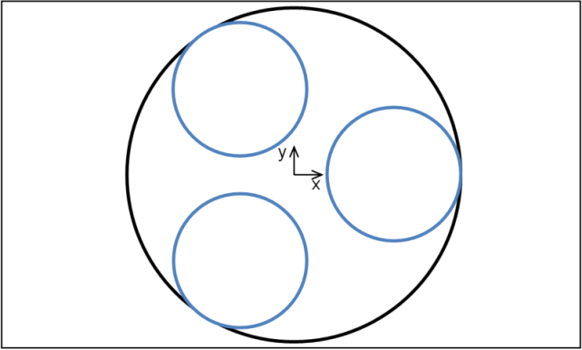
The centres of the blue inner lines are far away from the centre of the black outer lines and so singularity is avoided.
Discretisation is also possible – and useful – for around penetrators. This is illustrated below using a discretisation count of 3 and a discretisation scale of 1.6.

When modelling interference fits using line contact, the deficiencies of the undiscretised model are often very significant. The improvement to robustness and stability resulting from penetrator discretisation can be profound.
Torsion modelling for line contact splined lines
In the previous releases of OrcaFlex, splined lines for line contact required torsion to be included. Whilst torsion is modelled perfectly well by OrcaFlex, there are a couple of consequences:
- Simulation times when modelling torsion are somewhat slower than when excluding torsion. This is quite reasonable since including torsion doubles the number of degrees of freedom.
- Statics convergence for line contact is less robust when torsion is modelled.
One of the by-products of the line supports development is that we were able to relax the restrictions for splined lines to require torsion. So, for splined lines in line contact relationships that do not model friction, modelling of torsion is no longer required.
Models that are able to take advantage of this and exclude torsion modelling should see much improved statics convergence.
3DOF calculated vessels can be used with the implicit solver
One of the major development tasks that we have been working on recently has been a re-implementation of our low level solver. This has been motivated by the desire to be able to:
- Use the same solver for both implicit and explicit integration. At present in OrcaFlex, implicit integration, full statics and whole system statics are all handled by the same low level solver code. However, explicit integration is handled by legacy code that dates from the days before our implicit solver.
- Solve frequency domain problems.
- Solve non-spatial degrees of freedom, for instance the wake oscillator degree of freedom. The current implicit solver cannot do this and so wake oscillators are limited to explicit integration.
- Handle more general constraints. For example, to be able to suppress individual degrees of freedom, not restricted to degrees of freedom with respect to the global axes directions.
OrcaFlex 9.8 now uses the new solver, but we have not yet been able to realise any of the above goals! So, functionally this change brings few immediate benefits. Rather we are laying foundations for the future.
The exception to that statement is that the new solver allows us to remove the restriction that 3DOF vessel calculated primary motion was not available for the implicit solver. For version 9.8 this restriction has been removed. So, let this minor enhancement be a taster for the much more significant improvements that are to come!
Conclusion
So, that’s all folks, as the saying goes. We hope that you enjoy and appreciate this new version of OrcaFlex, and find good use for all the new features.