OrcaFlex has two objects whose motion can be imposed rather than calculated:

• The vessel object through displacement RAOs, harmonic motion, time history or externally calculated motion.
• The constraint object (added in version 10.1) through motion time histories in the constraint’s imposed displacement mode.

In addition to these more well-known methods of imposing motion, the constraint object has another mechanism that allows motion to be imposed.

OrcaFlex 10.2 extended the constraint object by adding the curvilinear constraint model. The typical usage of curvilinear constraints is to define one or more bespoke coordinates, and then express the Cartesian coordinates in terms of these user defined coordinates.

For instance, a Cartesian calculated constraint can constrain an object to lie along a straight line, a plane, etc. A curvilinear constraint can constrain an object to lie on arbitrary non-Cartesian curves and surfaces.

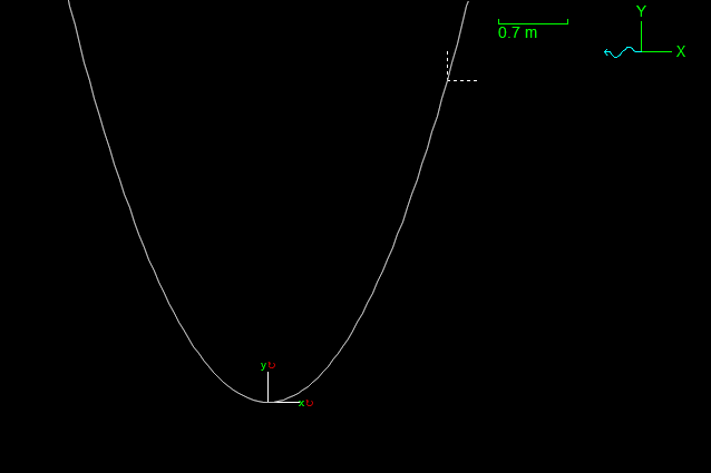
As an example, we show how to use a curvilinear constraint to constrain an object to lie on a parabola with equation \(y = x^2\). To do this, define a single free coordinate, \(q\) say, and then define the curvilinear mappings to be as follows:

x = q
y = x**2
z = 0
Rx = 0
Ry = 0
Rz = 0

The result looks like this:

All of the above leads to calculated motion, but we are interested in imposed motion. The trick is to use a curvilinear constraint with no free coordinates. By having no free coordinates we ensure that motion is not calculated, but how can we impose it? Well, OrcaFlex helpfully defines a number of other symbols which can be used to impose motion. These include:

• \(t\), the current simulation time
• \(t0\), the simulation time at the start of the simulation
• \(ramp\), the current value of the ramping factor

By defining the curvilinear mappings in terms of these symbols (principally time \(t\)) we are able to impose a motion. For example, consider the following mapping:

x = 0
y = 0
z = 0
Rx = 0
Ry = 0
Rz = t - t0

The idea is that \(Rz\), the rotation angle about the \(Z\) axis, varies linearly with time. The resulting simulation looks like this:

Whilst this example demonstrates the point reasonably well, it is not hard to produce identical behaviour using a time history imposed motion constraint. Perhaps more compelling is the following example where we impose a sinusoidal displacement on the constraint. The mapping is:

x = sin(t - t0)
y = 0
z = 0
Rx = 0
Ry = 0
Rz = 0

The result is as follows:

Again, this could be recreated with a time history imposed motion constraint but it would be much more labourious. We would need to tabulate the \(sin\) function to the same resolution as the model time step. Any change in simulation duration or time step would potentially force us to re-tabulate the function.

This is a rather niche subject area, but we hope that at least some of our users will find the methods here to be useful, if not today perhaps at some point in the future.