A year has elapsed since we released OrcaFlex 10.0, which means that it is time for the next version. We are very pleased to announce the 2016 release of OrcaFlex, version 10.1.

The software was finalised and built on 19^th October. We are currently preparing the installation program, and will then dispatch the software. All clients with up-to-date MUS contracts should receive the new version early in November.

Version 10.1 introduces much new functionality, including:

• Constraints, a new type of object that provide general purpose connections between objects. Constraints can be used to fix individual degrees of freedom (DOFs) and to impose displacements on individual DOFs.
• Enhancements to frequency domain analysis, particularly for calculated vessel responses at both low and wave frequencies.
• Mid-line connections – the ability to connect nodes in the middle of lines to other objects, just as is possible for nodes at the ends of lines.
• Improvements in multi-threaded performance on machines with more than 64 processors or with NUMA memory architecture.

These are the most significant developments, in our opinion. As always there are a great many more enhancements which are documented in the What’s New topic for 10.1.

What follows is a brief introduction to each of the new features that we consider to be of most significance.

Constraints

Constraints are a new type of object that provide an enhanced, versatile means of connecting objects. They can be used to:

• Fix individual DOFs.
• Introduce individual DOFs.
• Impose displacements on individual DOFs.

Constraints were developed primarily to enable simpler modelling of the following:

• Hinges and articulations.
• Telescoping joints.
• Crane operations.

This list is not intended to be exhaustive. Constraints can be applied in many other situations.

What are constraint objects?

A constraint object comprises two frames of reference: the in-frame and the out-frame. The in-frame is rigidly connected to a master object and therefore translates and rotates with the master object. Slaves of the constraint are rigidly connected to the out-frame and so translate and rotate with the out-frame. The out-frame can translate and rotate, independently in all six DOFs, relative to the in-frame, and it is this capability in particular that makes constraints so versatile and useful.

Typically, a constraint object will be used as a means to connect objects together. The constraint is connected to a master object (e.g. vessel, buoy, line, etc.), and has one or more objects connected as slaves. Constraint objects themselves have no physical properties such as mass or volume, and do not attract hydrodynamic or aerodynamic loading. Their utility is derived entirely from the out-frame’s ability to move relative to the in-frame.

There are two distinct modes of operation for constraints, Calculated DOFs and Imposed displacement. These two modes offer different ways of controlling the relative movement between the out-frame and the in-frame.

Calculated DOFs

Individual DOFs, three translational and three rotational, can be either calculated or fixed, as determined by the input data. For example, to specify a single rotational degree of freedom, about the local y-axis, as would be used to model a hinge, the input data would look like this:

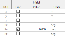
The column of check boxes titled Free is used to specify which DOFs are free and which are fixed. Different settings for these check boxes allow different types of connection to be modelled. For example, to model a telescoping joint you would make a single translational DOF be free.

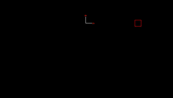
To demonstrate how the above data models a hinge, the animation below shows the constraint, with a buoy attached to provide mass, acting as a pendulum. The axes drawn with a solid pen represent the in-frame, fixed to global. The dashed axes represent the out-frame. The single degree of freedom is Ry, rotation about local y, where y is normal to the view.

Prior to the introduction of constraints, there were a variety of standard workarounds that could be used to model hinges, articulations, telescoping joints etc. For instance, hinges would usually have been modelled using very stiff single segment lines. But these workarounds were often tricky to build, and sometimes caused numerical problems. With the advent of constraints these issues become a thing of the past.

In addition, calculated constraints also allow specification of stiffness and damping, which can be linear or nonlinear. These properties can be used to resist displacement and velocity of the out-frame relative to the in-frame. Further, applied loads can be specified (constant, time varying, or externally calculated) and applied to the out-frame.

Imposed displacement

The original motivation for constraints was the Calculated DOFs mode. However, as that feature took shape we realised that these objects could be useful for other forms of connection / constraint. Thus were Imposed Displacement constraints born.

Before this release, the only object capable of imposing motion (as opposed to calculating motion) was the vessel. This could be done through prescribed motion, time history, or external calculation. Although it feels odd to use an OrcaFlex vessel as a means to impose motion, that sort of trick is quite common in OrcaFlex. However, the real weakness is that vessels cannot be connected as slaves of other objects. Constraints have no such limitation.

When imposed displacements are used, the displacement of the out-frame, relative to the in-frame, is specified by time history. All 6 degrees of freedom can be varied, or indeed any subset of the degrees of freedom.

There are many scenarios where imposed displacement constraints are useful. The ability to connect objects together in chains allows multiple imposed displacement constraints to be connected together to form a compound imposed motion. An example where that is especially useful is to model crane operations, as shown in this video:

Having given pre-release demonstrations of constraints to many users over the past few months, I can safely say that they have generated more excitement than any new feature since we added the implicit time domain solver. We hope you have as much fun with them as we have had!

Frequency domain dynamic analysis

In version 10.0, frequency domain dynamic analysis was added. This was the result of a huge development effort, and the sheer size of the program meant that some features were not initially supported in the frequency domain. The most important of these omitted features was calculated vessels. In version 10.1 we have addressed that omission and OrcaFlex now supports calculated vessels in the frequency domain.

There are really two distinct parts to this development, wave frequency and low frequency. The frequency domain functionality in version 10.0 caters for first order wave loading, what we refer to internally as the wave frequency solver. Extending this functionality to support first order wave load RAOs on vessels is relatively straightforward, and fits into the existing program quite naturally.

While enhancing the wave frequency solver to support calculated vessels presented few challenges, implementing low frequency analysis is a much more demanding task. This type of analysis is often used to study the low frequency response of moored systems to 2^nd order wave drift loading, and to wind loading. The normal solution method is quite different from that used by OrcaFlex’s wave frequency solver. We have developed a method of re-expressing the low frequency problem in a way that can be handled by the same underlying frequency domain solver code.

Using the same underlying solver code for both wave frequency and low frequency means that all result types and variables currently supported in the wave frequency solver are also available in the low frequency solver. Mooring line damping is linearised by the same frame invariant MMSE scheme employed at wave frequency. And finally, a less obvious but very important benefit of sharing the same solver is that any future development will be quicker and less prone to error.

These enhancements now mean that OrcaFlex has a frequency domain engine capable of performing mooring analysis in the frequency domain. However, this should really be considered a work in progress. While the solver is very capable, there are further enhancements that would make it easier to use:

• There is scope for much improved results presentation that targets mooring applications.
• We do not yet support non-Gaussian extreme statistics for the low frequency solver.
• The mechanics and workflow of defining and analysing all the load cases for a mooring analysis could be improved.

We feel that we have made a good start towards making OrcaFlex an effective tool for frequency domain mooring analysis and now have a powerful solver which we can build on and improve. We would really appreciate and encourage feedback to help guide us in making the next steps towards that goal. So, if you have interests in this area, we would love to hear from you and learn how you feel the program could be improved.

Mid-line connections

In recent releases we have added a number of features to make modelling of connections more flexible:

• Connecting lines to lines (version 10.0)
• Chains of connections, e.g. Buoy1 is connected to Buoy2, which in turn is connected to Buoy3 etc. (version 10.0)
• Constraint objects (version 10.1)

One notable limitation in all of this, is the ability to have connections at mid-line nodes. The nodes at each end of a line can be connected as slaves of other objects. But the other nodes in a line are always master of their degrees of freedom. Other objects can be connected as slaves of mid-line nodes, but mid-line nodes could not previously be masters.

That has changed with 10.1, very much driven by the desire to apply constraints to mid-line nodes. It is now possible to define mid-line connections, that is to specify that nodes away from the ends are slaves of other objects. By making a mid-line node slave to a constraint, we are able to constrain individual node DOFs. Imposed displacement constraints can be used to impose the motion of a mid-line node. Mid-line nodes can, of course, be connected to objects other than constraints. End nodes can be connected as slaves to constraints, thus allowing the same capabilities.

As a fun demonstration, the animation below shows a single line with the node at the mid-point connected to a constraint object. The constraint object introduces a single translational degree of freedom. The simulation was started with the mid-point node initially perturbed and then released at the start of dynamics. The resulting motion is, in essence, just like the pendulum above.

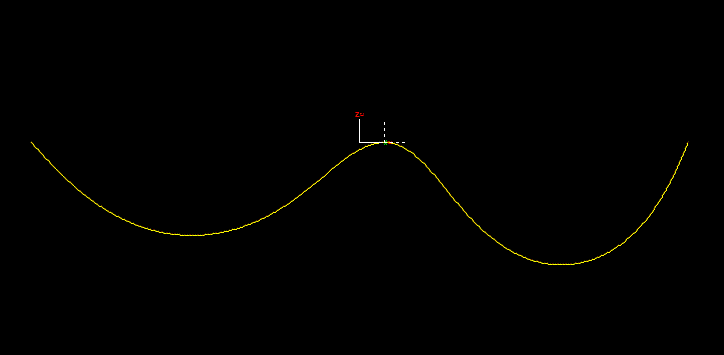
Obviously this is not intended to be an example of real-world OrcaFlex modelling, but it hopefully serves to illustrate the point. Without mid-line connections this model would have required two separate line objects, joined together at the constraint. Modelled with mid-line connections, a single line can be used, and more importantly, a single range graph plot can show the results for the entire line.

Multi-threaded performance on large machines

Way back in version 9.2 (released in 2008) the OrcaFlex batch functionality was extended to make use of all the processors on a machine. Before then jobs were processed in serial fashion. This was an excellent development, but as is so often the case, changes in computer hardware soon caught up with us. Machines with larger numbers of processors became available, and such machines come with complications:

• A naively written application, on Windows, cannot take advantage of more than 64 processors. Machines with more than 64 processors exist, and OrcaFlex was incapable of reaching all the processors.
• When a machine has a great many processors, shared memory access becomes more difficult to implement efficiently at the hardware level. This issue is typically addressed by using a non-uniform memory access (NUMA) design. On such machines, programs must typically be programmed to be aware of NUMA in order to perform well. Again, OrcaFlex was not aware of NUMA architecture and so could not extract the best performance from the machine.

In version 10.1, we have made changes to support machines with more than 64 processors, and to be aware of NUMA. As a result, OrcaFlex batch processing now scales much better on such machines.

The same issues affect Distributed OrcaFlex. Consequently, we are making similar changes to Distributed OrcaFlex and plan to release an updated version later this year.

The solution that we are opting for with Distributed OrcaFlex is to use multiple processes rather than multi-threading as used by OrcaFlex batch processing. One consequence of using multiple processes is much better scaling for Python external functions and post-calculation actions. So if you integrate Python code in that way you might find that the new Distributed OrcaFlex implementation is useful – even if you only want to process jobs on a single machine.

Conclusion

So, that’s OrcaFlex 10.1. We hope you enjoy it, and find good use for all the new features. We are already busy working on 10.2 which you can expect to see towards the end of 2017.